Linear Regression Using R: An Introduction to Data Modeling

(1)

LINEAR REGRESSION USING R

AN INTRODUCTION TO DATA

(2)

Linear Regression

Using R

A

N

I

NTRODUCTION TO

D

ATA

M

ODELING

D

AVID

J. L

ILJA

University of Minnesota, Minneapolis

(3)

Linear Regression Using R: An Introduction to Data Modeling Copyright c 2016 by David J. Lilja

This work is licensed under a Creative Commons Attribution-NonCommercial 4.0 International License. You are free to:

Share – copy and redistribute the material in any medium or format Adapt – remix, transform, and build upon the material

The licensor cannot revoke these freedoms as long as you follow the license terms. Under the following terms:

Attribution – You must give appropriate credit, provide a link to the license, and indicate if changes were made. You may do so in any reasonable manner, but not in any way that suggests the licensor endorses you or your use. NonCommercial – You may not use the material for commercial purposes.

Although every precaution has been taken to verify the accuracy of the information contained herein, the author and publisher assume no responsibility for any errors or omissions. No liability is assumed for damages that may result from the use of information contained within.

Edition: 1.1 (April, 2017) Edition: 1.0 (2016)

University of Minnesota Libraries Publishing Minneapolis, Minnesota, USA

ISBN-10: 1-946135-00-3 ISBN-13: 978-1-946135-00-1 https:/doi.org/10.24926/8668/1301 Visit the book web site at:

(4)

Preface

Goals

Interest in what has become popularly known as data mining has expanded significantly in the past few years, as the amount of data generated contin-ues to explode. Furthermore, computing systems’ ever-increasing capabil-ities make it feasible to deeply analyze data in ways that were previously available only to individuals with access to expensive, high-performance computing systems.

Learning about the broad field of data mining really means learning a range of statistical tools and techniques. Regression modeling is one of those fundamental techniques, while the R programming language is widely used by statisticians, scientists, and engineers for a broad range of statistical analyses. A working knowledge of R is an important skill for anyone who is interested in performing most types of data analysis.

The primary goal of this tutorial is to explain, in step-by-step detail, how to develop linear regression models. It uses a large, publicly available data set as a running example throughout the text and employs the R program-ming language environment as the computational engine for developing the models.

This tutorial will not make you an expert in regression modeling, nor a complete programmer in R. However, anyone who wants to understand how to extract information from data needs a working knowledge of the basic concepts used to develop reliable regression models, and should also know how to use R. The specific focus, casual presentation, and detailed examples will help you understand the modeling process, using R as your computational tool.

(5)

All of the resources you will need to work through the examples in the book are readily available on the book web site (see p.ii). Furthermore, a fully functional R programming environment is available as a free, open-source download [13].

Audience

Students taking university-level courses on data science, statistical model-ing, and related topics, plus professional engineers and scientists who want to learn how to perform linear regression modeling, are the primary audi-ence for this tutorial. This tutorial assumes that you have at least some ex-perience with programming, such as what you would typically learn while studying for any science or engineering degree. However, you do not need to be an expert programmer. In fact, one of the key advantages of R as a programming language for developing regression models is that it is easy to perform remarkably complex computations with only a few lines of code.

Acknowledgments

Writing a book requires a lot of time by yourself, concentrating on trying to say what you want to say as clearly as possible. But developing and publishing a book is rarely the result of just one person’s effort. This book is no exception.

At the risk of omitting some of those who provided both direct and in-direct assistance in preparing this book, I thank the following individuals for their help: Professor Phil Bones of the University of Canterbury in Christchurch, New Zealand, for providing me with a quiet place to work on this text in one of the most beautiful countries in the world, and for our many interesting conversations; Shane Nackerud and Kristi Jensen of the University of Minnesota Libraries for their logistical and financial support through the Libraries’ Partnership for Affordable Content grant program; and Brian Conn, also of the University of Minnesota Libraries, for his in-sights into the numerous publishing options available for this type of text, and for steering me towards the Partnership for Affordable Content pro-gram. I also want to thank my copy editor, Ingrid Case, for gently and tact-fully pointing out my errors and inconsistencies. Any errors that remain are

(6)

my own fault, most likely because I ignored Ingrid’s advice. Finally, none of this would have happened without Sarah and her unwavering support.

Without these people, this book would be just a bunch of bits, moldering away on a computer disk drive somewhere.

(7)

(8)

Introduction

D

ATA mining is a phrase that has been popularly used to suggest the

process of finding useful information from within a large collection of data. I like to think of data mining as encompassing a broad range of statistical techniques and tools that can be used to extract different types of information from your data. Which particular technique or tool to use depends on your specific goals.

One of the most fundamental of the broad range of data mining

tech-niques that have been developed isregression modeling. Regression

mod-eling is simply generating a mathematical model from measured data. This

model is said toexplainan output value given a new set of input values.

Linear regression modelingis a specific form of regression modeling that assumes that the output can be explained using a linear combination of the input values.

A common goal for developing a regression model is to predict what the output value of a system should be for a new set of input values, given that you have a collection of data about similar systems. For example, as you gain experience driving a car, you begun to develop an intuitive sense of how long it might take you to drive somewhere if you know the type of car, the weather, an estimate of the traffic, the distance, the condition of the roads, and so on. What you really have done to make this estimate of driving time is constructed a multi-factor regression model in your mind. The inputs to your model are the type of car, the weather, etc. The output is how long it will take you to drive from one point to another. When you change any of the inputs, such as a sudden increase in traffic, you automatically re-estimate how long it will take you to reach the destination. This type of model building and estimating is precisely what we are

(11)

CHAPTER 1. INTRODUCTION

ing to learn to do more formally in this tutorial. As a concrete example, we will use real performance data obtained from thousands of measurements of computer systems to develop a regression model using the R statisti-cal software package. You will learn how to develop the model and how to evaluate how well it fits the data. You also will learn how to use it to predict the performance of other computer systems.

As you go through this tutorial, remember that what you are developing is just a model. It will hopefully be useful in understanding the system and in predicting future results. However, do not confuse a model with the real system. The real system will always produce the correct results, regardless of what the model may say the results should be.

1.1

||

What is a Linear Regression Model?

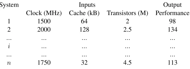
Suppose that we have measured the performance of several different com-puter systems using some standard benchmark program. We can organize these measurements into a table, such as the example data shown in

Ta-ble1.1. The details of each system are recorded in a single row. Since we

measured the performance ofndifferent systems, we neednrows in the

[image:11.432.67.370.372.482.2]

table.

Table 1.1: An example of computer system performance data.

System Inputs Output

Clock (MHz) Cache (kB) Transistors (M) Performance

1 1500 64 2 98

2 2000 128 2.5 134

... ... ... ... ...

i ... ... ... ...

... ... ... ... ...

n 1750 32 4.5 113

The first column in this table is the index number (or name) from 1 ton

that we have arbitrarily assigned to each of the different systems measured.

Columns 2-4 are theinput parameters. These are called theindependent

variablesfor the system we will be modeling. The specific values of the

(12)

1.1. WHAT IS A LINEAR REGRESSION MODEL?

input parameters were set by the experimenter when the system was mea-sured, or they were determined by the system configuration. In either case, we know what the values are and we want to measure the performance obtained for these input values. For example, in the first system, the cessor’s clock was 1500 MHz, the cache size was 64 kbytes, and the pro-cessor contained 2 million transistors. The last column is the performance that was measured for this system when it executed a standard benchmark

program. We refer to this value as the outputof the system. More

tech-nically, this is known as the system’s dependent variableor the system’s

response.

The goal of regression modeling is to use these n independent

mea-surements to determine a mathematical function, f(), that describes the

relationship between the input parameters and the output, such as:

perf ormance=f(Clock, Cache, T ransistors) (1.1)

This function, which is just an ordinary mathematical equation, is the regression model. A regression model can take on any form. However, we will restrict ourselves to a function that is a linear combination of the input parameters. We will explain later that, while the function is a linear combination of the input parameters, the parameters themselves do not need to be linear. This linear combination is commonly used in regression modeling and is powerful enough to model most systems we are likely to encounter.

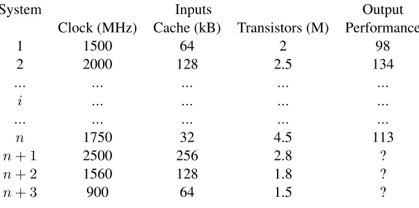
In the process of developing this model, we will discover how impor-tant each of these inputs are in determining the output value. For example, we might find that the performance is heavily dependent on the clock fre-quency, while the cache size and the number of transistors may be much less important. We may even find that some of the inputs have essentially no impact on the output making it completely unnecessary to include them in the model. We also will be able to use the model we develop to predict the performance we would expect to see on a system that has input values that did not exist in any of the systems that we actually measured. For

instance, Table 1.2shows three new systems that were not part of the set

of systems that we previously measured. We can use our regression model to predict the performance of each of these three systems to replace the question marks in the table.

(13)

[image:13.432.67.368.123.273.2]

CHAPTER 1. INTRODUCTION

Table 1.2: An example in which we want to predict the performance of new

systemsn+ 1,n+ 2, andn+ 3using the previously measured

results from the othernsystems.

System Inputs Output

Clock (MHz) Cache (kB) Transistors (M) Performance

1 1500 64 2 98

2 2000 128 2.5 134

... ... ... ... ...

i ... ... ... ...

... ... ... ... ...

n 1750 32 4.5 113

n+ 1 2500 256 2.8 ?

n+ 2 1560 128 1.8 ?

n+ 3 900 64 1.5 ?

As a final point, note that, since the regression model is a linear com-bination of the input values, the values of the model parameters will auto-matically be scaled as we develop the model. As a result, the units used for the inputs and the output are arbitrary. In fact, we can rescale the values of the inputs and the output before we begin the modeling process and still produce a valid model.

1.2

||

What is R?

R is a computer language developed specifically for statistical computing. It is actually more than that, though. R provides a complete environment for interacting with your data. You can directly use the functions that are provided in the environment to process your data without writing a com-plete program. You also can write your own programs to perform opera-tions that do not have built-in funcopera-tions, or to repeat the same task multiple times, for instance.

R is an object-oriented language that uses vectors and matrices as its ba-sic operands. This feature makes it quite useful for working on large sets of data using only a few lines of code. The R environment also provides

(14)

1.2. WHAT IS R?

cellent graphical tools for producing complex plots relatively easily. And, perhaps best of all, it is free. It is an open source project developed by many volunteers. You can learn more about the history of R, and

down-load a copy to your own computer, from the R Project web site [13].

As an example of using R, here is a copy of a simple interaction with the R environment.

> x <- c(2,4,6,8,10,12,14,16) > x

[1] 2 4 6 8 10 12 14 16 > mean(x)

[1] 9 > var(x) [1] 24 >

In this listing, the “>” character indicates that R is waiting for input. The linex <- c(2, 4, 6, 8, 10, 12, 14, 16)concatenates all of the values in the argument into a vector and assigns that vector to the variablex. Simply

typingxby itself causes R to print the contents of the vector. Note that R

treats vectors as a matrix with a single row. Thus, the “[1]” preceding the values is R’s notation to show that this is the first row of the matrixx. The

next line,mean(x), calls a function in R that computes the arithmetic mean

of the input vector, x. The function var(x)computes the corresponding

variance.

This book will not make you an expert in programming using the R computer language. Developing good regression models is an interactive process that requires you to dig in and play around with your data and your models. Thus, I am more interested in using R as a computing environment for doing statistical analysis than as a programming language. Instead of teaching you the language’s syntax and semantics directly, this tutorial will introduce what you need to know about R as you need it to perform the spe-cific steps to develop a regression model. You should already have some programming expertise so that you can follow the examples in the remain-der of the book. However, you do not need to be an expert programmer.

(15)

CHAPTER 1. INTRODUCTION

1.3

||

What’s Next?

Before beginning any sort of data analysis, you need to understand your

data. Chapter2describes the sample data that will be used in the examples

throughout this tutorial, and how to read this data into the R environment.

Chapter3introduces the simplest regression model consisting of a single

independent variable. The process used to develop a more complex re-gression model with multiple independent input variables is explained in

Chapter4. Chapter 5then shows how to use this multi-factor regression

model to predict the system response when given new input data. Chap-ter6explains in more detail the routines used to read a file containing your data into the R environment. The process used to develop a multi-factor

regression model is summarized in Chapter7along with some suggestions

for further reading. Finally, Chapter 8 provides some experiments you

might want to try to expand your understanding of the modeling process.

(16)

2

|

Understand Your Data

G

OODdata is the basis of any sort of regression model, because we use

this data to actually construct the model. If the data is flawed, the

model will be flawed. It is the old maxim of garbage in, garbage out.

Thus, the first step in regression modeling is to ensure that your data is reliable. There is no universal approach to verifying the quality of your data, unfortunately. If you collect it yourself, you at least have the advan-tage of knowing its provenance. If you obtain your data from somewhere else, though, you depend on the source to ensure data quality. Your job then becomes verifying your source’s reliability and correctness as much as possible.

2.1

||

Missing Values

Any large collection of data is probably incomplete. That is, it is likely that there will be cells without values in your data table. These missing values may be the result of an error, such as the experimenter simply for-getting to fill in a particular entry. They also could be missing because that particular system configuration did not have that parameter available. For example, not every processor tested in our example data had an L2 cache. Fortunately, R is designed to gracefully handle missing values. R uses the notationNAto indicate that the corresponding value is not available.

Most of the functions in R have been written to appropriately ignoreNA

values and still compute the desired result. Sometimes, however, you must

explicitly tell the function to ignore the NA values. For example, calling

the mean()function with an input vector that containsNAvalues causes it

to return NAas the result. To compute the mean of the input vector while

(17)

CHAPTER 2. UNDERSTAND YOUR DATA

ignoring theNAvalues, you must explicitly tell the function to remove the

NAvalues usingmean(x, na.rm=TRUE).

2.2

||

Sanity Checking and Data Cleaning

Regardless of where you obtain your data, it is important to do somesanity

checksto ensure that nothing is drastically flawed. For instance, you can check the minimum and maximum values of key input parameters (i.e., columns) of your data to see if anything looks obviously wrong. One of

the exercises in Chapter8 encourages you explore other approaches for

verifying your data. R also provides good plotting functions to quickly obtain a visual indication of some of the key relationships in your data set.

We will see some examples of these functions in Section3.1.

If you discover obvious errors or flaws in your data, you may have to eliminate portions of that data. For instance, you may find that the perfor-mance reported for a few system configurations is hundreds of times larger than that of all of the other systems tested. Although it is possible that this data is correct, it seems more likely that whoever recorded the data simply made a transcription error. You may decide that you should delete those results from your data. It is important, though, not to throw out data that looks strange without good justification. Sometimes the most interesting conclusions come from data that on first glance appeared flawed, but was actually hiding an interesting and unsuspected phenomenon. This process of checking your data and putting it into the proper format is often called

data cleaning.

It also is always appropriate to use your knowledge of the system and the relationships between the inputs and the output to inform your model building. For instance, from our experience, we expect that the clock rate will be a key parameter in any regression model of computer systems per-formance that we construct. Consequently, we will want to make sure that our models include the clock parameter. If the modeling methodology sug-gests that the clock is not important in the model, then using the method-ology is probably an error. We additionally may have deeper insights into the physical system that suggest how we should proceed in developing a model. We will see a specific example of applying our insights about the effect of caches on system performance when we begin constructing more

(18)

2.3. THE EXAMPLE DATA

complex models in Chapter4.

These types of sanity checks help you feel more comfortable that your data is valid. However, keep in mind that it is impossible to prove that your data is flawless. As a result, you should always look at the results of any regression modeling exercise with a healthy dose of skepticism and think carefully about whether or not the results make sense. Trust your intuition. If the results don’t feel right, there is quite possibly a problem lurking somewhere in the data or in your analysis.

2.3

||

The Example Data

I obtained the input data used for developing the regression models in the

subsequent chapters from the publicly available CPU DB database [2].

This database contains design characteristics and measured performance results for a large collection of commercial processors. The data was col-lected over many years and is nicely organized using a common format and a standardized set of parameters. The particular version of the database used in this book contains information on 1,525 processors.

Many of the database’s parameters (columns) are useful in understand-ing and comparunderstand-ing the performance of the various processors. Not all of these parameters will be useful as predictors in the regression models, how-ever. For instance, some of the parameters, such as the column labeled

Instruction set width, are not available for many of the processors.

Oth-ers, such as theProcessor family, are common among several processors

and do not provide useful information for distinguishing among them. As a result, we can eliminate these columns as possible predictors when we develop the regression model.

On the other hand, based on our knowledge of processor design, we know that the clock frequency has a large effect on performance. It also seems likely that the parallelism-related parameters, specifically, the num-ber of threads and cores, could have a significant effect on performance, so we will keep these parameters available for possible inclusion in the regression model.

Technology-related parameters are those that are directly determined by the particular fabrication technology used to build the processor. The num-ber of transistors and the die size are rough indicators of the size and

(19)

CHAPTER 2. UNDERSTAND YOUR DATA

plexity of the processor’s logic. The feature size, channel length, and FO4 (fanout-of-four) delay are related to gate delays in the processor’s logic. Because these parameters both have a direct effect on how much process-ing can be done per clock cycle and effect the critical path delays, at least some of these parameters could be important in a regression model that describes performance.

Finally, the memory-related parameters recorded in the database are the separate L1 instruction and data cache sizes, and the unified L2 and L3 cache sizes. Because memory delays are critical to a processor’s perfor-mance, all of these memory-related parameters have the potential for being important in the regression models.

The reported performance metric is the score obtained from the SPEC CPU integer and floating-point benchmark programs from 1992, 1995,

2000, and 2006 [6–8]. This performance result will be the regression

model’s output. Note that performance results are not available for every processor running every benchmark. Most of the processors have perfor-mance results for only those benchmark sets that were current when the processor was introduced into the market. Thus, although there are more than 1,500 lines in the database representing more than 1,500 unique pro-cessor configurations, a much smaller number of results are reported for each individual benchmark.

2.4

||

Data Frames

The fundamental object used for storing tables of data in R is called adata frame. We can think of a data frame as a way of organizing data into a large table with a row for each system measured and a column for each parameter. An interesting and useful feature of R is that all the columns in a data frame do not need to be the same data type. Some columns may consist of numerical data, for instance, while other columns contain textual data. This feature is quite useful when manipulating large, heterogeneous data files.

To access the CPU DB data, we first must read it into the R environ-ment. R has built-in functions for reading data directly from files in the

csv(comma separated values) format and for organizing the data into data

frames. The specifics of this reading process can get a little messy,

(20)

2.4. DATA FRAMES

ing on how the data is organized in the file. We will defer the specifics of

reading the CPU DB file into R until Chapter 6. For now, we will use a

function calledextract_data(), which was specifically written for reading

the CPU DB file.

To use this function, copy both theall-data.csv andread-data.Rfiles

into a directory on your computer (you can download both of these files

from this book’s web site shown on p. ii). Then start the R environment

and set the local directory in R to be this directory using theFile -> Change

dirpull-down menu. Then use theFile -> Source R codepull-down menu

to read theread-data.Rfile into R. When the R code in this file completes,

you should have six new data frames in your R environment workspace: int92.dat,fp92.dat,int95.dat,fp95.dat,int00.dat,fp00.dat,int06.dat,

andfp06.dat.

The data frameint92.datcontains the data from the CPU DB database

for all of the processors for which performance results were available for

the SPEC Integer 1992 (Int1992) benchmark program. Similarly,fp92.dat

contains the data for the processors that executed the Floating-Point 1992

(Fp1992) benchmarks, and so on. I use the .datsuffix to show that the

corresponding variable name is a data frame.

Simply typing the name of the data frame will cause R to print the en-tire table. For example, here are the first few lines printed after I type int92.dat, truncated to fit within the page:

nperf perf clock threads cores ...

1 9.662070 68.60000 100 1 1 ...

2 7.996196 63.10000 125 1 1 ...

3 16.363872 90.72647 166 1 1 ...

4 13.720745 82.00000 175 1 1 ...

...

The first row is the header, which shows the name of each column. Each subsequent row contains the data corresponding to an individual processor. The first column is the index number assigned to the processor whose data is in that row. The next columns are the specific values recorded for that

parameter for each processor. The functionhead(int92.dat)prints out just

the header and the first few rows of the corresponding data frame. It gives you a quick glance at the data frame when you interact with your data.

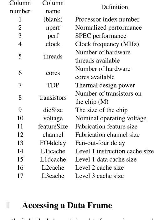
Table 2.1shows the complete list of column names available in these

(21)

CHAPTER 2. UNDERSTAND YOUR DATA

[image:21.432.87.333.150.502.2]

data frames. Note that the column names are listed vertically in this table, simply to make them fit on the page.

Table 2.1: The names and definitions of the columns in the data frames containing the data from CPU DB.

Column number

Column

name Definition

1 (blank) Processor index number

2 nperf Normalized performance

3 perf SPEC performance

4 clock Clock frequency (MHz)

5 threads Number of hardware

threads available

6 cores Number of hardware

cores available

7 TDP Thermal design power

8 transistors Number of transistors on

the chip (M)

9 dieSize The size of the chip

10 voltage Nominal operating voltage

11 featureSize Fabrication feature size

12 channel Fabrication channel size

13 FO4delay Fan-out-four delay

14 L1icache Level 1 instruction cache size

15 L1dcache Level 1 data cache size

16 L2cache Level 2 cache size

17 L3cache Level 3 cache size

2.5

||

Accessing a Data Frame

We access the individual elements in a data frame using square brackets to identify a specific cell. For instance, the following accesses the data in the cell in row 15, column 12:

(22)

2.5. ACCESSING A DATA FRAME

> int92.dat[15,12] [1] 180

We can also access cells by name by putting quotes around the name:

> int92.dat["71","perf"] [1] 105.1

This expression returns the data in the row labeled 71and the column

labeledperf. Note that this is not row 71, but rather the row that contains the data for the processor whose name is71.

We can access an entire column by leaving the first parameter in the square brackets empty. For instance, the following prints the value in every

row for the column labeledclock:

> int92.dat[,"clock"] [1] 100 125 166 175 190 ...

Similarly, this expression prints the values in all of the columns for row 36:

> int92.dat[36,]

nperf perf clock threads cores ...

36 13.07378 79.86399 80 1 1 ...

The functionsnrow()andncol()return the number of rows and columns,

respectively, in the data frame:

> nrow(int92.dat) [1] 78

> ncol(int92.dat) [1] 16

Because R functions can typically operate on a vector of any length, we can use built-in functions to quickly compute some useful results. For ex-ample, the following expressions compute the minimum, maximum, mean,

and standard deviation of theperfcolumn in theint92.datdata frame:

> min(int92.dat[,"perf"]) [1] 36.7

> max(int92.dat[,"perf"]) [1] 366.857

> mean(int92.dat[,"perf"]) [1] 124.2859

> sd(int92.dat[,"perf"]) [1] 78.0974

(23)

CHAPTER 2. UNDERSTAND YOUR DATA

This square-bracket notation can become cumbersome when you do a substantial amount of interactive computation within the R environment.

R provides an alternative notation using the$symbol to more easily access

a column. Repeating the previous example using this notation:

> min(int92.dat$perf) [1] 36.7

> max(int92.dat$perf) [1] 366.857

> mean(int92.dat$perf) [1] 124.2859

> sd(int92.dat$perf) [1] 78.0974

This notation says to use the data in the column namedperffrom the data

frame namedint92.dat. We can make yet a further simplification using the

attachfunction. This function makes the corresponding data frame local to

the current workspace, thereby eliminating the need to use the potentially

awkward$ or square-bracket indexing notation. The following example

shows how this works:

> attach(int92.dat) > min(perf)

[1] 36.7 > max(perf) [1] 366.857 > mean(perf) [1] 124.2859 > sd(perf) [1] 78.0974

To change to a different data frame within your local workspace, you must firstdetachthe current data frame:

> detach(int92.dat) > attach(fp00.dat) > min(perf) [1] 87.54153 > max(perf) [1] 3369 > mean(perf) [1] 1217.282 > sd(perf) [1] 787.4139

Now that we have the necessary data available in the R environment, and some understanding of how to access and manipulate this data, we are

(24)

2.5. ACCESSING A DATA FRAME

ready to generate our first regression model.

(25)

(26)

3

|

One-Factor Regression

T

HEsimplest linear regression model finds the relationship between one

input variable, which is called thepredictorvariable, and the output,

which is called the system’s response. This type of model is known as

a one-factor linear regression. To demonstrate the regression-modeling process, we will begin developing a one-factor model for the SPEC Integer 2000 (Int2000) benchmark results reported in the CPU DB data set. We will expand this model to include multiple input variables in Chapter4.

3.1

||

Visualize the Data

The first step in this one-factor modeling process is to determine whether or not itlooksas though a linear relationship exists between the predictor and the output value. From our understanding of computer system design - that

is, from ourdomain-specific knowledge- we know that the clock frequency

strongly influences a computer system’s performance. Consequently, we must look for a roughly linear relationship between the processor’s per-formance and its clock frequency. Fortunately, R provides powerful and flexible plotting functions that let us visualize this type relationship quite easily.

This R function call:

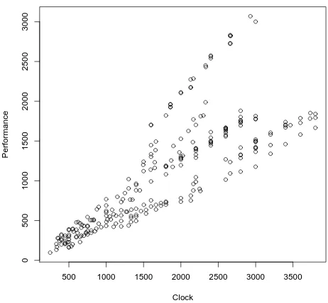
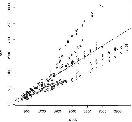
> plot(int00.dat[,"clock"],int00.dat[,"perf"], main="Int2000", xlab="Clock", ylab="Performance")

generates the plot shown in Figure 3.1. The first parameter in this

func-tion call is the value we will plot on the x-axis. In this case, we will plot theclockvalues from theint00.datdata frame as the independent variable

(27)

CHAPTER 3. ONE-FACTOR REGRESSION

500 1000 1500 2000 2500 3000 3500

[image:27.432.100.331.71.285.2]

0 5 0 0 1 0 0 0 1 5 0 0 2 0 0 0 2 5 0 0 3 0 0 0 Int2000 Clock P e rf o rm a n c e

Figure 3.1: A scatter plot of the performance of the processors that were tested using the Int2000 benchmark versus the clock frequency.

on the x-axis. The dependent variable is theperfcolumn fromint00.dat,

which we plot on the y-axis. The function argumentmain="Int2000" pro-vides a title for the plot, whilexlab="Clock"andylab="Performance" pro-vide labels for the x- and y-axes, respectively.

This figure shows that the performance tends to increase as the clock fre-quency increases, as we expected. If we superimpose a straight line on this scatter plot, we see that the relationship between the predictor (the clock frequency) and the output (the performance) is roughly linear. It is not per-fectly linear, however. As the clock frequency increases, we see a larger spread in performance values. Our next step is to develop a regression model that will help us quantify the degree of linearity in the relationship between the output and the predictor.

(28)

3.2. THE LINEAR MODEL FUNCTION

3.2

||

The Linear Model Function

We use regression models to predict a system’s behavior by extrapolating from previously measured output values when the system is tested with known input parameter values. The simplest regression model is a straight line. It has the mathematical form:

y=a0+a1x1 (3.1)

wherex1 is the input to the system,a0is the y-intercept of the line,a1 is the slope, andyis the output value the model predicts.

R provides the functionlm()that generates a linear model from the data

contained in a data frame. For this one-factor model, R computes the

val-ues of a0 and a1 using the method of least squares. This method finds

the line that most closely fits the measured data by minimizing the dis-tances between the line and the individual data points. For the data frame

int00.dat, we compute the model as follows:

> attach(int00.dat)

> int00.lm <- lm(perf ~ clock)

The first line in this example attaches the int00.datdata frame to the

current workspace. The next line calls the lm()function and assigns the

resultinglinear model object to the variable int00.lm. We use the suffix

.lmto emphasize that this variable contains a linear model. The argument

in the lm()function, (perf ~ clock), says that we want to find a model

where the predictorclockexplains the outputperf.

Typing the variable’s name,int00.lm, by itself causes R to print the

ar-gument with which the functionlm()was called, along with the computed

coefficients for the regression model.

> int00.lm

Call:

lm(formula = perf ~ clock)

Coefficients:

(Intercept) clock

51.7871 0.5863

In this case, the y-intercept isa0 = 51.7871and the slope isa1 = 0.5863. Thus, the final regression model is:

(29)

CHAPTER 3. ONE-FACTOR REGRESSION

500 1000 1500 2000 2500 3000 3500

0

5

0

1

0

1

5

0

2

0

2

5

0

3

0

clock

p

e

[image:29.432.102.331.74.285.2]

rf

Figure 3.2: The one-factor linear regression model superimposed on the data from Figure3.1.

perf = 51.7871 + 0.5863∗clock. (3.2)

The following code plots the original data along with the fitted line, as shown in Figure3.2. The functionabline()is short for(a,b)-line. It plots a line on the active plot window, using the slope and intercept of the linear model given in its argument.

> plot(clock,perf) > abline(int00.lm)

3.3

||

Evaluating the Quality of the Model

The information we obtain by typing int00.lm shows us the regression

model’s basic values, but does not tell us anything about the model’s qual-ity. In fact, there are many different ways to evaluate a regression model’s

(30)

3.3. EVALUATING THE QUALITY OF THE MODEL

quality. Many of the techniques can be rather technical, and the details of

them are beyond the scope of this tutorial. However, the functionsummary()

extracts some additional information that we can use to determine how well the data fit the resulting model. When called with the model object int00.lmas the argument,summary()produces the following information:

> summary(int00.lm)

Call:

Residuals:

Min 1Q Median 3Q Max

-634.61 -276.17 -30.83 75.38 1299.52

Coefficients:

Estimate Std. Error t value Pr(>|t|) (Intercept) 51.78709 53.31513 0.971 0.332 clock 0.58635 0.02697 21.741 <2e-16 ***

---Signif. codes: 0 ‘***’ 0.001 ‘**’ 0.01 ‘*’ 0.05 ‘.’ 0.1 ‘ ’ 1

Residual standard error: 396.1 on 254 degrees of freedom Multiple R-squared: 0.6505, Adjusted R-squared: 0.6491 F-statistic: 472.7 on 1 and 254 DF, p-value: < 2.2e-16

Let’s examine each of the items presented in this summary in turn.

> summary(int00.lm)

Call:

These first few lines simply repeat how thelm()function was called. It

is useful to look at this information to verify that you actually called the function as you intended.

Residuals:

-634.61 -276.17 -30.83 75.38 1299.52

Theresidualsare the differences between the actual measured values and

the corresponding values on the fitted regression line. In Figure3.2, each

data point’s residual is the distance that the individual data point is above

(positive residual) or below (negative residual) the regression line. Minis

the minimum residual value, which is the distance from the regression line

(31)

CHAPTER 3. ONE-FACTOR REGRESSION

to the point furthest below the line. Similarly,Maxis the distance from the

regression line of the point furthest above the line. Medianis the median

value of all of the residuals. The1Qand3Qvalues are the points that mark the first and third quartiles of all the sorted residual values.

How should we interpret these values? If the line is a good fit with the data, we would expect residual values that are normally distributed around a mean of zero. (Recall that a normal distribution is also called a Gaussian distribution.) This distribution implies that there is a decreasing probability of finding residual values as we move further away from the mean. That is, a good model’s residuals should be roughly balanced around and not too far away from the mean of zero. Consequently, when we look at the

residual values reported bysummary(), a good model would tend to have

a median value near zero, minimum and maximum values of roughly the same magnitude, and first and third quartile values of roughly the same magnitude. For this model, the residual values are not too far off what we

would expect for Gaussian-distributed numbers. In Section3.4, we present

a simple visual test to determine whether the residuals appear to follow a normal distribution.

Coefficients:

Estimate Std. Error t value Pr(>|t|) (Intercept) 51.78709 53.31513 0.971 0.332 clock 0.58635 0.02697 21.741 <2e-16 ***

---Signif. codes: 0 ‘***’ 0.001 ‘**’ 0.01 ‘*’ 0.05 ‘.’ 0.1 ‘ ’ 1

This portion of the output shows the estimated coefficient values. These

values are simply the fitted regression model values from Equation 3.2.

TheStd. Errorcolumn shows the statisticalstandard errorfor each of the coefficients. For a good model, we typically would like to see a standard error that is at least five to ten times smaller than the corresponding

coeffi-cient. For example, the standard error forclockis 21.7 times smaller than

the coefficient value (0.58635/0.02697 = 21.7). This large ratio means that there is relatively little variability in the slope estimate,a1. The standard error for the intercept,a0, is 53.31513, which is roughly the same as the es-timated value of 51.78709 for this coefficient. These similar values suggest that the estimate of this coefficient for this model can vary significantly.

The last column, labeledPr(>|t|), shows the probability that the

corre-sponding coefficient isnotrelevant in the model. This value is also known

(32)

3.3. EVALUATING THE QUALITY OF THE MODEL

as thesignificanceorp-value of the coefficient. In this example, the prob-ability thatclockis not relevant in this model is2×10−16 - a tiny value. The probability that the intercept is not relevant is 0.332, or about a one-in-three chance that this specific intercept value is not relevant to the model. There is an intercept, of course, but we are again seeing indications that the model is not predicting this value very well.

The symbols printed to the right in this summary - that is, the asterisks, periods, or spaces - are intended to give a quick visual check of the

coeffi-cients’ significance. The line labeledSignif. codes:gives these symbols’

meanings. Three asterisks (***) means0< p≤0.001, two asterisks (**)

means0.001< p≤0.01, and so on.

R uses the column labeledt valueto compute thep-values and the

cor-responding significance symbols. You probably will not use these values directly when you evaluate your model’s quality, so we will ignore this column for now.

Residual standard error: 396.1 on 254 degrees of freedom Multiple R-squared: 0.6505, Adjusted R-squared: 0.6491 F-statistic: 472.7 on 1 and 254 DF, p-value: < 2.2e-16

These final few lines in the output provide some statistical information

about the quality of the regression model’s fit to the data. TheResidual

standard error is a measure of the total variation in the residual values.

If the residuals are distributed normally, the first and third quantiles of the previous residuals should be about 1.5 times this standard error.

The number ofdegrees of freedomis the total number of measurements

or observations used to generate the model, minus the number of coeffi-cients in the model. This example had 256 unique rows in the data frame, corresponding to 256 independent measurements. We used this data to pro-duce a regression model with two coefficients: the slope and the intercept. Thus, we are left with (256 - 2 = 254) degrees of freedom.

TheMultiple R-squaredvalue is a number between 0 and 1. It is a statis-tical measure of how well the model describes the measured data. We com-pute it by dividing the total variation that the model explains by the data’s total variation. Multiplying this value by 100 gives a value that we can

interpret as a percentage between 0 and 100. The reportedR2 of 0.6505

for this model means that the model explains 65.05 percent of the data’s variation. Random chance and measurement errors creep in, so the model

(33)

CHAPTER 3. ONE-FACTOR REGRESSION

will never explain all data variation. Consequently, you should not ever expect anR2_{value of exactly one. In general, values of}_R2_{that are closer} to one indicate a better-fitting model. However, a good model does not necessarily require a largeR2value. It may still accurately predict future

observations, even with a smallR2value.

TheAdjusted R-squaredvalue is theR2value modified to take into

ac-count the number of predictors used in the model. The adjusted R2 is

always smaller than theR2value. We will discuss the meaining of the

ad-justedR2 in Chapter4, when we present regression models that use more

than one predictor.

The final line shows theF-statistic. This value compares the current

model to a model that has one fewer parameters. Because the one-factor model already has only a single parameter, this test is not particularly use-ful in this case. It is an interesting statistic for the multi-factor models, however, as we will discuss later.

3.4

||

Residual Analysis

Thesummary() function provides a substantial amount of information to help us evaluate a regression model’s fit to the data used to develop that model. To dig deeper into the model’s quality, we can analyze some addi-tional information about the observed values compared to the values that the model predicts. In particular,residual analysisexamines these residual values to see what they can tell us about the model’s quality.

Recall that the residual value is the difference between the actual mea-sured value stored in the data frame and the value that the fitted regression line predicts for that corresponding data point. Residual values greater than zero mean that the regression model predicted a value that was too small compared to the actual measured value, and negative values indicate that the regression model predicted a value that was too large. A model that fits the data well would tend to over-predict as often as it under-predicts. Thus, if we plot the residual values, we would expect to see them distributed uniformly around zero for a well-fitted model.

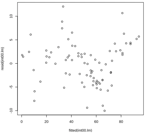
The following function calls produce the residuals plot for our model, shown in Figure3.3.

> plot(fitted(int00.lm),resid(int00.lm))

(34)

3.4. RESIDUAL ANALYSIS

500 1000 1500 2000

-5

0

5

0

1

0

fitted(int00.lm)

re

s

id

(i

n

t0

0

.l

m

[image:34.432.98.328.101.315.2]

)

Figure 3.3: The residual values versus the input values for the one-factor model developed using the Int2000 data.

In this plot, we see that the residuals tend to increase as we move to the right. Additionally, the residuals are not uniformly scattered above and below zero. Overall, this plot tells us that using the clock as the sole predictor in the regression model does not sufficiently or fully explain the data. In general, if you observe any sort of clear trend or pattern in the residuals, you probably need to generate a better model. This does not mean that our simple one-factor model is useless, though. It only means that we may be able to construct a model that produces tighter residual values and better predictions.

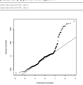
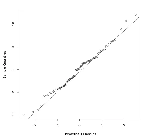
Another test of the residuals uses thequantile-versus-quantile, orQ-Q, plot. Previously we said that, if the model fits the data well, we would expect the residuals to be normally (Gaussian) distributed around a mean of zero. The Q-Q plot provides a nice visual indication of whether the residuals from the model are normally distributed. The following function

(35)

CHAPTER 3. ONE-FACTOR REGRESSION

calls generate the Q-Q plot shown in Figure3.4:

> qqnorm(resid(int00.lm)) > qqline(resid(int00.lm))

-3 -2 -1 0 1 2 3

-5

0

5

0

1

0

Normal Q-Q Plot

Theoretical Quantiles

S

a

m

p

le

Q

u

a

n

ti

le

[image:35.432.84.351.74.348.2]

s

Figure 3.4: The Q-Q plot for the one-factor model developed using the Int2000 data.

If the residuals were normally distributed, we would expect the points plotted in this figure to follow a straight line. With our model, though, we see that the two ends diverge significantly from that line. This behavior indicates that the residuals are not normally distributed. In fact, this plot suggests that the distribution’s tails are “heavier” than what we would ex-pect from a normal distribution. This test further confirms that using only the clock as a predictor in the model is insufficient to explain the data.

Our next step is to learn to develop regression models with multiple input factors. Perhaps we will find a more complex model that is better able to explain the data.

(36)

4

|

Multi-factor Regression

A

multi-factor regression model is a generalization of the simple one-factor regression model discussed in Chapter3. It hasnfactors with the form:

y=a0+a1x1+a2x2+...anxn, (4.1)

where thexivalues are the inputs to the system, theaicoefficients are the

model parameters computed from the measured data, and yis the output

value predicted by the model. Everything we learned in Chapter3for

one-factor models also applies to the multi-one-factor models. To develop this type of multi-factor regression model, we must also learn how to select specific predictors to include in the model

4.1

||

Visualizing the Relationships in the Data

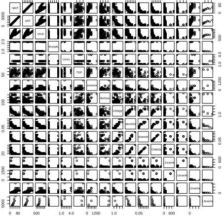
Before beginning model development, it is useful to get a visual sense of the relationships within the data. We can do this easily with the following function call:

> pairs(int00.dat, gap=0.5)

The pairs() function produces the plot shown in Figure 4.1. This plot

provides a pairwise comparison of all the data in theint00.datdata frame.

The gap parameter in the function call controls the spacing between the

individual plots. Set it to zero to eliminate any space between plots. As an example of how to read this plot, locate the box near the upper left

corner labeledperf. This is the value of the performance measured for the

int00.datdata set. The box immediately to the right of this one is a scatter

(37)

CHAPTER 4. MULTI-FACTOR REGRESSION

nperf

0 3000 1.0 2.0 50 100 0.05 20 0 1500 5000

0 8 0 0 3 0 0 0 perf clock 5 0 0 1 .0 2 .0 threads cores 1 .0 4 .0 5 0 TDP transistors 0 1 2 0 0 1 0 0 dieSize voltage 1 .0 0 .0 5 featureSize channel 0 .0 5 2 0 FO4delay L1icache 0 6 0 0 0 1 5 0 0 L1dcache L2cache 0 0 80 5 0 0 0

[image:37.432.109.336.64.282.2]

500 1.0 4.0 0 1200 1.0 0.05 0 600 0 L3cache

Figure 4.1: All of the pairwise comparisons for the Int2000 data frame.

plot, withperfdata on the vertical axis andclockdata on the horizontal

axis. This is the same information we previously plotted in Figure3.1. By

scanning through these plots, we can see any obviously significant relation-ships between the variables. For example, we quickly observe that there is

a somewhat proportional relationship betweenperfand clock. Scanning

down theperfcolumn, we also see that there might be a weakly inverse

relationship betweenperfandfeatureSize.

Notice that there is a perfect linear correlation betweenperfandnperf.

This relationship occurs becausenperfis a simple rescaling ofperf. The

reported benchmark performance values in the database - that is, theperf

values - use different scales for different benchmarks. To directly compare the values that our models will predict, it is useful to rescaleperfto the range [0,100]. Do this quite easily, using this R code:

max_perf = max(perf) min_perf = min(perf) range = max_perf - min_perf

nperf = 100 * (perf - min_perf) / range

(38)

4.2. IDENTIFYING POTENTIAL PREDICTORS

Note that this rescaling has no effect on the models we will develop, be-cause it is a linear transformation ofperf. For convenience and consistency, we usenperfin the remainder of this tutorial.

4.2

||

Identifying Potential Predictors

The first step in developing the multi-factor regression model is to identify all possible predictors that we could include in the model. To the novice model developer, it may seem that we should include all factors available in the data as predictors, because more information is likely to be better than not enough information. However, a good regression model explains the relationship between a system’s inputs and output as simply as pos-sible. Thus, we should use the smallest number of predictors necessary to provide good predictions. Furthermore, using too many or redundant predictors builds the random noise in the data into the model. In this

sit-uation, we obtain anover-fittedmodel that is very good at predicting the

outputs from the specific input data set used to train the model. It does

not accurately model the overall system’s response, though, and it will not appropriately predict the system output for a broader range of inputs than those on which it was trained. Redundant or unnecessary predictors also can lead to numerical instabilities when computing the coefficients.

We must find a balance between including too few and too many predic-tors. A model with too few predictors can produce biased predictions. On the other hand, adding more predictors to the model will always cause the

R2value to increase. This can confuse you into thinking that the additional predictors generated a better model. In some cases, adding a predictor will

improve the model, so the increase in theR2value makes sense. In some

cases, however, theR2value increases simply because we’ve better

mod-eled the random noise.

TheadjustedR2 attempts to compensate for the regularR2’s behavior

by changing the R2 value according to the number of predictors in the

model. This adjustment helps us determine whether adding a predictor improves the fit of the model, or whether it is simply modeling the noise

(39)

CHAPTER 4. MULTI-FACTOR REGRESSION

better. It is computed as:

R2_adjusted= 1− n−1

n−m(1−R

2

) (4.2)

wherenis the number of observations andmis the number of predictors

in the model. If adding a new predictor to the model increases the previous

model’sR2_{value by more than we would expect from random fluctuations,}

then the adjustedR2will increase. Conversely, it will decrease if removing

a predictor decreases theR2by more than we would expect due to random

variations. Recall that the goal is to use as few predictors as possible, while still producing a model that explains the data well.

Because we do not knowa prioriwhich input parameters will be useful

predictors, it seems reasonable to start with all of the columns available in the measured data as the set of potential predictors. We listed all of

the column names in Table2.1. Before we throw all these columns into

the modeling process, though, we need to step back and consider what we know about the underlying system, to help us find any parameters that we should obviously exclude from the start.

There are two output columns: perf andnperf. The regression model

can have only one output, however, so we must choose only one column to

use in our model development process. As discussed in Section4.1,nperf

is a linear transformation ofperfthat shifts the output range to be between 0 and 100. This range is useful for quickly obtaining a sense of future

predictions’ quality, so we decide to usenperfas our model’s output and

ignore theperfcolumn.

Almost all the remaining possible predictors appear potentially useful in our model, so we keep them available as potential predictors for now.

The only exception isTDP. The name of this factor,thermal design power,

does not clearly indicate whether this could be a useful predictor in our model, so we must do a little additional research to understand it

bet-ter. We discover [10] that thermal design power is “the average amount

of power in watts that a cooling system must dissipate. Also called the ‘thermal guideline’ or ‘thermal design point,’ the TDP is provided by the chip manufacturer to the system vendor, who is expected to build a case that accommodates the chip’s thermal requirements.” From this definition, we conclude thatTDPis not really a parameter that will directly affect

(40)

4.2. IDENTIFYING POTENTIAL PREDICTORS

formance. Rather, it is a specification provided by the processor’s manu-facturer to ensure that the system designer includes adequate cooling capa-bility in the final product. Thus, we decide not to includeTDPas a potential predictor in the regression model.

In addition to excluding some apparently unhelpful factors (such as TDP) at the beginning of the model development process, we also should con-sider whether we should include any additional parameters. For example, the terms in a regression model add linearly to produce the predicted out-put. However, the individual terms themselves can be nonlinear, such as

aixm_i , wheremdoes not have to be equal to one. This flexibility lets us

in-clude additional powers of the individual factors. We should inin-clude these non-linear terms, though, only if we have some physical reason to suspect that the output could be a nonlinear function of a particular input.

For example, we know from our prior experience modeling processor performance that empirical studies have suggested that cache miss rates

are roughly proportional to the square root of the cache size [5].

Con-sequently, we will include terms for the square root (m = 1/2) of each

cache size as possible predictors. We must also include first-degree terms

(m= 1) of each cache size as possible predictors. Finally, we notice that

only a few of the entries in theint00.datdata frame include values for the

L3 cache, so we decide to exclude the L3 cache size as a potential pre-dictor. Exploiting this type of domain-specific knowledge when selecting predictors ultimately can help produce better models than blindly applying the model development process.

The final list of potential predictors that we will make available for the

model development process is shown in Table4.1.

Table 4.1: The list of potential predictors to be used in the model develop-ment process.

clock threads cores transistors

dieSize voltage f eatureSize channel

F O4delay_√ L1icache √L1icache L1dcache

L1dcache L2cache √L2cache

(41)

CHAPTER 4. MULTI-FACTOR REGRESSION

4.3

||

The Backward Elimination Process

We are finally ready to develop the multi-factor linear regression model for theint00.datdata set. As mentioned in the previous section, we must find the right balance in the number of predictors that we use in our model. Too many predictors will train our model to follow the data’s random variations (noise) too closely. Too few predictors will produce a model that may not be as accurate at predicting future values as a model with more predictors.

We will use a process called backward elimination [1] to help decide

which predictors to keep in our model and which to exclude. In backward

elimination, we start with all possible predictors and then uselm()to

com-pute the model. We use the summary()function to find each predictor’s

significance level. The predictor with the least significance has the largest

p-value. If this value is larger than our predetermined significance thresh-old, we remove that predictor from the model and start over. A typical threshold for keeping predictors in a model isp= 0.05, meaning that there is at least a 95 percent chance that the predictor is meaningful. A threshold

ofp = 0.10also is not unusual. We repeat this process until the

signifi-cance levels of all of the predictors remaining in the model are below our threshold.

Note that backward elimination is not the only approach to developing

regression models. A complementary approach is forward selection. In

this approach, we successively add potential predictors to the regression model as long as their significance levels in the computed model remain below the predefined threshold. This process continues, one at a time for each potential predictor, until all of the predictors have been tested. Other approaches includestep-wise regression,all possible regressions, and au-tomated selectionapproaches.

All of these approaches have their advantages and disadvantages, their supporters and detractors. I prefer the backward elimination process be-cause it is usually straightforward to determine which factor we should drop at each step of the process. Determining which factor to try at each step is more difficult with forward selection. Backward elimination has a further advantage, in that several factors together may have better pre-dictive power than any subset of these factors. As a result, the backward elimination process is more likely to include these factors as a group in the

(42)

4.4. AN EXAMPLE OF THE BACKWARD ELIMINATION PROCESS

final model than is the forward selection process.

The automated procedures have a very strong allure because, as techno-logically savvy individuals, we tend to believe that this type of automated process will likely test a broader range of possible predictor combinations than we could test manually. However, these automated procedures lack intuitive insights into the underlying physical nature of the system being modeled. Intuition can help us answer the question of whether this is a reasonable model to construct in the first place.

As you develop your models, continually ask yourself whether the model

“makes sense.” Does it make sense that factor i is included but factorj

is excluded? Is there a physical explanation to support the inclusion or exclusion of any potential factor? Although the automated methods can simplify the process, they also make it too easy for you to forget to think about whether or not each step in the modeling process makes sense.

4.4

||

An Example of the Backward Elimination

Process

We previously identified the list of possible predictors that we can include

in our models, shown in Table4.1. We start the backward elimination

pro-cess by putting all these potential predictors into a model for theint00.dat

data frame using thelm()function.

> int00.lm <- lm(nperf ~ clock + threads + cores + transistors + dieSize + voltage + featureSize + channel + FO4delay + L1icache + sqrt(L1icache) + L1dcache + sqrt(L1dcache) + L2cache + sqrt(L2cache), data=int00.dat)

This function call assigns the resulting linear model object to the variable

int00.lm. As before, we use the suffix.lmto remind us that this variable

is a linear model developed from the data in the corresponding data frame, int00.dat. The arguments in the function call telllm()to compute a linear

model that explains the outputnperfas a function of the predictors

sepa-rated by the “+” signs. The argumentdata=int00.datexplicitly passes to

thelm()function the name of the data frame that should be used when

de-veloping this model. Thisdata=argument is not necessary if weattach()

the data frameint00.datto the current workspace. However, it is useful to

(43)

CHAPTER 4. MULTI-FACTOR REGRESSION

explicitly specify the data frame thatlm()should use, to avoid confusion

when you manipulate multiple models simultaneously.

Thesummary()function gives us a great deal of information about the linear model we just created:

> summary(int00.lm)

Call:

lm(formula = nperf ~ clock + threads + cores + transistors + dieSize + voltage + featureSize + channel + FO4delay + L1icache + sqrt(L1icache) + L1dcache + sqrt(L1dcache) + L2cache + sqrt(L2cache), data = int00.dat)

Residuals:

-10.804 -2.702 0.000 2.285 9.809

Coefficients:

Estimate Std. Error t value Pr(>|t|) (Intercept) -2.108e+01 7.852e+01 -0.268 0.78927 clock 2.605e-02 1.671e-03 15.594 < 2e-16 *** threads -2.346e+00 2.089e+00 -1.123 0.26596 cores 2.246e+00 1.782e+00 1.260 0.21235 transistors -5.580e-03 1.388e-02 -0.402 0.68897 dieSize 1.021e-02 1.746e-02 0.585 0.56084 voltage -2.623e+01 7.698e+00 -3.408 0.00117 ** featureSize 3.101e+01 1.122e+02 0.276 0.78324 channel 9.496e+01 5.945e+02 0.160 0.87361 FO4delay -1.765e-02 1.600e+00 -0.011 0.99123 L1icache 1.102e+02 4.206e+01 2.619 0.01111 * sqrt(L1icache) -7.390e+02 2.980e+02 -2.480 0.01593 * L1dcache -1.114e+02 4.019e+01 -2.771 0.00739 ** sqrt(L1dcache) 7.492e+02 2.739e+02 2.735 0.00815 ** L2cache -9.684e-03 1.745e-03 -5.550 6.57e-07 *** sqrt(L2cache) 1.221e+00 2.425e-01 5.034 4.54e-06 ***

---Signif. codes: 0 ‘***’ 0.001 ‘**’ 0.01 ‘*’ 0.05 ‘.’ 0.1 ‘ ’ 1

Residual standard error: 4.632 on 61 degrees of freedom (179 observations deleted due to missingness)

Multiple R-squared: 0.9652, Adjusted R-squared: 0.9566 F-statistic: 112.8 on 15 and 61 DF, p-value: < 2.2e-16

Notice a few things in this summary: First, a quick glance at the residu-als shows that they are roughly balanced around a median of zero, which is what we like to see in our models. Also, notice the line,(179 observations deleted due to missingness). This tells us that in 179 of the rows in the

data frame - that is, in 179 of the processors for which performance

(44)

4.4. AN EXAMPLE OF THE BACKWARD ELIMINATION PROCESS

sults were reported for the Int2000 benchmark - some of the values in the columns that we would like to use as potential predictors were missing.

TheseNA values caused R to automatically remove these data rows when

computing the linear model.

The total number of observations used in the model equals the number of degrees of freedom remaining - 61 in this case - plus the total number of predictors in the model. Finally, notice that theR2and adjustedR2values

are relatively close to one, indicating that the model explains the nperf

values well. Recall, however, that these largeR2values may simply show

us that the model is good at modeling the noise in the measurements. We must still determine whether we should retain all these potential predictors in the model.

To continue developing the model, we apply the backward elimination procedure by identifying the predictor with the largestp-value that exceeds

our predetermined threshold ofp= 0.05. This predictor isFO4delay, which

has ap-value of 0.99123. We can use theupdate()function to eliminate a

given predictor and recompute the model in one step. The notation “.~.”

means thatupdate()should keep the left- and right-hand sides of the model

the same. By including “- FO4delay,” we also tell it to remove that predic-tor from the model, as shown in the following:

> int00.lm <- update(int00.lm, .~. - FO4delay, data = int00.dat) > summary(int00.lm)

Call:

lm(formula = nperf ~ clock + threads + cores + transistors + dieSize + voltage + featureSize + channel + L1icache + sqrt(L1icache) + L1dcache + sqrt(L1dcache) + L2cache + sqrt(L2cache), data = int00.dat)

Residuals:

-10.795 -2.714 0.000 2.283 9.809

Coefficients:

Estimate Std. Error t value Pr(>|t|) (Intercept) -2.088e+01 7.584e+01 -0.275 0.783983 clock 2.604e-02 1.563e-03 16.662 < 2e-16 *** threads -2.345e+00 2.070e+00 -1.133 0.261641 cores 2.248e+00 1.759e+00 1.278 0.206080 transistors -5.556e-03 1.359e-02 -0.409 0.684020 dieSize 1.013e-02 1.571e-02 0.645 0.521488 voltage -2.626e+01 7.302e+00 -3.596 0.000642 *** featureSize 3.104e+01 1.113e+02 0.279 0.781232

(45)

CHAPTER 4. MULTI-FACTOR REGRESSION

channel 8.855e+01 1.218e+02 0.727 0.469815 L1icache 1.103e+02 4.041e+01 2.729 0.008257 ** sqrt(L1icache) -7.398e+02 2.866e+02 -2.581 0.012230 * L1dcache -1.115e+02 3.859e+01 -2.889 0.005311 ** sqrt(L1dcache) 7.500e+02 2.632e+02 2.849 0.005937 ** L2cache -9.693e-03 1.494e-03 -6.488 1.64e-08 *** sqrt(L2cache) 1.222e+00 1.975e-01 6.189 5.33e-08 ***

---Signif. codes: 0 ‘***’ 0.001 ‘**’ 0.01 ‘*’ 0.05 ‘.’ 0.1 ‘ ’ 1

We repeat this process by removing the next potential predictor with

the largestp-value that exceeds our predetermined threshold,featureSize.

As we repeat this process, we obtain the following sequence of possible models.

RemovefeatureSize:

> int00.lm <- update(int00.lm, .~. - featureSize, data=int00.dat) > summary(int00.lm)

Call:

lm(formula = nperf ~ clock + threads + cores + transistors + dieSize + voltage + channel + L1icache + sqrt(L1icache) + L1dcache + sqrt(L1dcache) + L2cache + sqrt(L2cache), data = int00.dat)

Residuals:

-10.5548 -2.6442 0.0937 2.2010 10.0264

Coefficients:

Estimate Std. Error t value Pr(>|t|) (Intercept) -3.129e+01 6.554e+01 -0.477 0.634666 clock 2.591e-02 1.471e-03 17.609 < 2e-16 *** threads -2.447e+00 2.022e+00 -1.210 0.230755 cores 1.901e+00 1.233e+00 1.541 0.128305 transistors -5.366e-03 1.347e-02 -0.398 0.691700 dieSize 1.325e-02 1.097e-02 1.208 0.231608 voltage -2.519e+01 6.182e+00 -4.075 0.000131 *** channel 1.188e+02 5.504e+01 2.158 0.034735 * L1icache 1.037e+02 3.255e+01 3.186 0.002246 ** sqrt(L1icache) -6.930e+02 2.307e+02 -3.004 0.003818 ** L1dcache -1.052e+02 3.106e+01 -3.387 0.001223 ** sqrt(L1dcache) 7.069e+02 2.116e+02 3.341 0.001406 ** L2cache -9.548e-03 1.390e-03 -6.870 3.37e-09 *** sqrt(L2cache) 1.202e+00 1.821e-01 6.598 9.96e-09 ***

(46)

4.4. AN EXAMPLE OF THE BACKWARD ELIMINATION PROCESS

---Signif. codes: 0 ‘***’ 0.001 ‘**’ 0.01 ‘*’ 0.05 ‘.’ 0.1 ‘ ’ 1

Removetransistors:

> int00.lm <- update(int00.lm, .~. - transistors, data=int00.dat) > summary(int00.lm)

Call:

lm

Linear Regression Using R: An Introduction to Data Modeling