Melitz in GTAP Made Easy: The A2M Conversion
Method and Result Interpretation
CoPS Working Paper No. G-284, July 2018
The Centre of Policy Studies (CoPS), incorporating the IMPACT project, is a research centre at Victoria University devoted to quantitative analysis of issues relevant to economic policy. Address: Centre of Policy Studies, Victoria University, PO Box 14428, Melbourne, Victoria, 8001 home page: www.vu.edu.au/CoPS/ email: [email protected] Telephone +61 3 9919 1877
Peter B. Dixon
And
Maureen T. Rimmer
Centre of Policy Studies, Victoria University
1
Melitz in GTAP made easy: the A2M conversion method and result interpretation
by
Peter B. Dixon and Maureen T. Rimmer
Centre of Policy Studies, Victoria University, Melbourne July 30, 2018
Abstract:
Since the 1970s the Armington approach has been the workhorse specification of trade in CGE models. Under Armington, agents substitute between products from different countries. Conceptually, Melitz provides a more attractive approach in which substitution is between products from different firms, rather than countries. Other attractive features of Melitz are allowance for: monopolistic competition; and economies of scale from fixed establishment costs for firms and fixed set-up costs on trade links. In this paper we show how an
Armington model can be converted to Melitz by adding a few equations and introducing closure swaps, with little change to existing code. We apply our Armington-to-Melitz method to the Armington-based GTAP model to derive GTAP-A2M. Then we show how results from a CGE model with Melitz industries can be interpreted and justified via back-of-the-envelope calculations. Finally, we review the strengths and weaknesses of GTAP-HET, an alternative Melitz-based version of GTAP.
Key words: heterogeneous firms; Armington to Melitz; GTAP-A2M; GTAP-HET; result interpretation
2
Melitz in GTAP made easy: the A2M conversion method and result interpretation
July 30, 2018
1. Introduction
In this paper we describe briefly:
(1) how an existing Armington-based model such as standard GTAP can be converted easily to a model with Melitz industries by the addition of some elementary equations and the use of closure swaps. We refer to the conversion method as Armington-to-Melitz, or A2M.
(2)how results from a mixed Armington-Melitz model can be explained.
(3)the relationship between GTAP-A2M and GTAP-HET created by Akgul, Villoria and Hertel (AVH, 2016).
The paper is brief because to a large extent it is a summary of material in Dixon, Jerie and Rimmer (DJR, 2018) which contains all of the underlying technical material together with instructions for downloading the GEMPACK code for the GTAP-A2M model.
2. The A2M conversion method
The GTAP model (Hertel, 1997)1 has been in constant use for more than 20 years. Its database is the outcome of an enormous world-wide cooperative effort organized by Tom Hertel and his colleagues at Purdue University. Because GTAP is used intensively for policy analyses it contains many unavoidable complications in the treatments of taxes, tariffs, technologies, trade flows, capital flows and capital accumulation. Thousands of economists are familiar with GTAP and many have completed courses on its Armington-based theory2, data and application. In short, there is a huge world-wide investment by economists in GTAP.
In these circumstances, achieving widespread adoption of a Melitz version3 of GTAP with new theory or data structures has the potential to impose large human-capital costs on the world’s community policy modellers. Thus, in introducing Melitz to GTAP, we looked for a method that would leave the theory and data structures of the standard GTAP model
essentially unchanged. We wanted to give users the opportunity to adopt Melitz assumptions in a model consisting of familiar GTAP plus a small number of add-on equations. We designed these add-on equation so that through closure swaps they could be turned on or off to introduce Melitz assumption for user-chosen industries.
1 The latest documentation of the GTAP model is Corong et al. (2017).
2 This is the theory introduced by Armington (1969) of imperfect substitution between commodities identified
by country of origin.
3 This refers to the theory set out by Melitz (2003) which incorporates monopolistic competition, fixed costs in
3
2.1. Preliminary modifications to standard GTAP
It was not possible to entirely avoid modifications to the GTAP model.4 We made five, none of which alter the fundamental theory of the standard Armington-based model, and none of which were difficult to implement. The five modifications are as follows.
Modification 1. We eliminated the difference between import-import substitution elasticities (ESUBM) and import-domestic substitution elasticities (ESUBD), effectively eliminating GTAP’s two-tier treatment of substitution between domestic and imported goods. This is necessary for Melitz sectors because in Melitz theory substitutability between any pair of varieties is the same as that between any other pair, irrespective of the varieties’ countries of origin. While the two-tier system is effectively eliminated, no substantive alteration is required to the GTAP code. We simply introduced a formula that made the values of ESUBM equal to those of ESUBD, overruling the initially read values of ESUBM.
Modification 2. Standard GTAP includes the variable ams(c,s,d) that allows for input-saving technical change in country d in the use of commodity c imported from country s. There is no corresponding variable that allows for input-saving technical change in the use of domestically-produced commodity c. We added such a variable, ads(c,s), taking care to include it where necessary in GTAP equations for: the demand by agents in country s for domestically produced commodity c; the cost to agents in country s of composite units of commodity c; and definitions of welfare and aggregate technical change. As we will see shortly, we need ads(c,s) as well as ams(c,s,d) to allow for the Melitz theory of love of variety.
Modification 3. In standard GTAP, the cost of transporting a unit of commodity c between countries s and d depends on the quantity transported and the cost of a unit of transport services. Consequently, changes in production costs in country s can affect the ratio of fob to cif prices for c sent from s to d. This is inconsistent with the iceberg view of trade costs favored by Melitz and other theorists. To implement Melitz theory accurately in GTAP, we added code that allows trade costs for selected commodities to be ad valorem. For these commodities, fob and cif prices can move by the same percentages. With this additional code, the ad valorem treatment for selected commodities can be implemented via closure swaps.
Modification 4. We added four new variables to standard GTAP: aoMel(c,s), txMel(c,s,d), pmarket(c,s,d) and pbundle(c,s). The first of these, aoMel(c,s), allows for increases in output per input bundle (to be defined shortly) used in industry c in country s. There is already a variable in standard GTAP [aoall(c,s)] that can play this role. Including aoMel(c,s) is simply a matter of convenience. It gives us a dedicated variable for implementing endogenous movements, consistent with Melitz theory, in total-factor productivity for Melitz industries. For Armington industries, aoMel(c,s) is exogenous on zero.
The second new variable, txMel(c,s,d), is the percentage change in the power of a tax applying to sales of commodity c flowing from s to d. Standard GTAP includes a variable that could play this role [the negative of txs(c,s,d)].5 Again, duplication is convenient. It gives us a dedicated variable, a Melitz tax, for implementing the Melitz theory of pricing to market. Along with txMel(c,s,d), we added to standard GTAP a variable and an equation for the collection of revenue [d_revtxMel(c,s,d)] from the Melitz tax on each commodity flow. As we will see, for a Melitz industry (c,s) the total collection added over destinations d of the
4 We worked with GTAP model 6.2 implemented with database 7.0 (November 2008). We chose the database
with 57 commodities and 10 regions.
4
Melitz taxes is set exogenously on zero. If c is an Armington industry, txMel(c,s,d) is exogenous on zero for all d.
Standard GTAP includes the variable pm(c,s) defined as the market price of commodity c produced in s. We don’t change the mathematical specification of pm(c,s). It continues to be the percentage change in the cost per unit of output of commodity c in country s. However we now refer to pm(c,s) as the percentage change in the factory price of (c,s). We reserve the expression “market price” for the cost just beyond the factory door of commodity (c,s)
destined for a specific country d. These destination-specific prices are denoted by pmarket(c,s,d). They differ from factory prices by the variable txMel(c,s,d), that is
pmarket(c,s, d)pm(c,s) txMel(c,s, d) (1)
Having added equation (1) to standard GTAP, we checked every place that pm appeared in the original GTAP code to see if it should remain as a factory price (pm) or be changed to a market price (pmarket).
The final new variable, pbundle(c,s), is the percentage change in the cost of the standard bundle of inputs required in industry (c,s). In the original Melitz theory, each industry used only one input, labor. In this case pbundle(c,s) is the percentage change in the wage rate in country s. In our GTAP-A2M system, pbundle(c,s) is percentage change in an index of input prices (modified by input-saving technical changes)6 with weights reflecting input shares in production in industry (c,s). With pm(c,s) being the percentage change in the cost per unit of output of commodity c in country s and with aoMel(c,s) being the percentage change in the output per input bundle we arrive at:
pm(c,s)pbundle(c,s) aoMel(c,s) (2)
Modification 5. The database for standard GTAP includes non-zero intra-regional trade flows, VXMD(c,s,s). These are the result of aggregation of countries to form regions. In creating our A2M system for GTAP, we treat regions as countries. Thus, non-zero values for VXMD(c,s,s) are awkward to handle. We chose to zero them out after adding them to
domestic demand, VMD(c,s). This procedure leaves balance conditions intact.
2.2. Additional equations to implement Melitz theory
In this subsection we describe the equations that we added to the end of the modified GTAP code to form the GTAP-A2M system. The first of these equations is:
qs(c,s, d)numl(c,s, d) qtypical(c,s, d) (3)
where
qs(c,s,d) is the percentage change in the quantity of commodity c sent from s to d. In GTAP notation qs(c,s,s) corresponds to qds(c,s) and qs(c,s,d) for d≠s corresponds to qxs(c,s,d).
numl(c,s,d) and qtypical(c,s,d) are Melitz concepts. They are the percentage changes in the number of c-producing firms in s that trade on the s,d-link and the quantity sent on the link by the typical, or average, (c,s) firm among those that trade on the link.7
6 While fixing ideas, it is easiest to think of pbundle(c,s) in a situation in which there are no changes in
input-saving technology: in GTAP terms, ams, ava, afe, af, aosec, aoreg, aoall and our new variable ads are set on zero. However, movements in these technology variables are taken into account in the determination of pbundle(c,s) with weights reflecting the share in (c,s)’s costs of the input on which the technical change operates.
5
The second add-on equation is:
txMel(c,s, d)aoMel(c,s) ptivity(c,s, d) f _ txMel(c,s, d) (4)
where
ptivity(c,s,d) is another Melitz concept. It is the percentage change in the marginal productivity of the typical c-producing firm on the s,d-link. By marginal productivity we mean the extra output produced for a unit increase in input. In Melitz theory, changes in the marginal productivity of the typical firm are not caused by productivity changes for any individual firm. Rather they reflect changes in the membership of the group of c-producing firms that are able to trade on the s,d-link.
f_txMel(c,s,d) is a shift variable. If c is an Armington industry, then this variable is endogenous and equation (4) is effectively eliminated. If c is a Melitz industry then the shift variable is exogenous on zero. In this case (4) in combination with (1) and (2) implies that
pmarket(c,s, d)pbundle(c,s) ptivity(c,s, d) (5)
Equation (5) gives us Melitz’ pricing to market.
To handle Melitz’ specification of love of variety we introduce the equation:
1
as(c,s, d) * numl(c,s, d) f _ as(c,s, d)
1 (c)
(6)
where
as(c,s,d) is the percentage change in the (c,s)-augmenting technology or preference variable for all agents in country d. In GTAP notation, as(c,s,d) for d≠s corresponds to ams(c,s,d). as(c,s,s) corresponds to our new variable ads(c,s).
f_as(c,s,d) is a shift variable, endogenous if c is an Armington industry and exogenous on zero if c is a Melitz industry.
(c) is elasticity of substitution between varieties of commodity c. In GTAP notation this corresponds to ESUBM(c), which we have assumed is the same as ESUBD(c).
In Melitz theory, (c) > 1. Thus the coefficient on numl(c,s,d) in (6) is positive. This means that increases in the number of c-producing firms on the s,d-link, which in Melitz theory is an increase in variety on the s,d-link, allows users in country d to achieve any given production or utility level with a smaller quantity count of c from s and no change in any other input.
6
d d d qbundle(c, s) (c) 1* SMV(c, s, d) * qs(c, s, d) ptivity(c, s, d) (c)
(c, s) (c) 1
* SMV(c, s, d) * numl(c, s, d) ff (c, s, d) (c, s) * (c)
(c) 1
* SMV(c, s, d) * num(c, s) hf (c, s)) (c, s) * (c)
fqbundle(c, s)
(7) whereSMV(c,s,d) is the share of industry (c,s)’s total costs represented by the market value of commodity (c,s) sent to d. In GTAP notation, this is VXMD(c,s,d)/VOM(c,s) for d≠s and VDM(c,s)/VOM(c,s) for d=s. The SMV(c,s,d)s sum over d to 1. For Armington
industries this reflects the GTAP assumption that the total market value of sales equals total costs. But what about Melitz industries where we allow for the Melitz tax,
txMel(c,s,d), to come between costs and market values? As mentioned earlier, for Melitz industries we fix the total collection of Melitz taxes on sales of industry (c,s) at zero. Thus, it remains true that the sum of (c,s)’s sales at market value equals (c,s)’s total costs.
num(c,s) is the Melitz variable giving the percentage change in the number of (c,s) firms.
hf(c,s) and ff(c,s,d) are the percentage changes in the Melitz variables for the number of input bundles required to set up a (c,s) firm and the number of input bundles for a (c,s) firm to set up trading on the s,d-link. These will normally be exogenous and shocked only in simulations concerned with the effects of changes in set-up technologies.
(c,s) is the shape parameter for the Pareto distribution of marginal productivity levels that we assume for (c,s) firms. It is a positive parameter whose value is greater than
(c) - 1.
fqbundle(c,s) is a shift variable, endogenous if c is an Armington industry and exogenous on zero if c is a Melitz industry.
A key assumption in the derivation of (7) is that the input composition of fixed costs in industry (c,s), that is the inputs required to set up firms and open trade links, is the same as that in current production. This assumption is avoided in GTAP-HET, see section 4. However, it has considerable simplifying benefits. Most obviously, it allows us to use a uniquely defined input bundle for industry (c,s).
While the derivation of equation (7) is too long for inclusion here8, the ideas behind it are transparent.
The first idea is that under Melitz assumptions, the mark up on variable costs is the same fraction, ((c)-1)/(c), of the market value of all of industry (c,s)’s sales. For example, if
8 Readers who would like to work through the derivation are referred to Chapter 4 in DJR (2018), particularly
7
(c) = 3, then 2/3rds of the market value of (c,s)’s sales on the s,d-link is the cost of input bundles required to produce (c,s)’s product for supply on the s,d-link. Thus, the share of industry (c,s)’s total purchase of input bundles (or total costs) accounted for by variable costs to supply the s,d-link is (2/3)*SMV(c,s,d). This explains the first term on the RHS of (7):if sales on the s,d-link increase by 10 per cent [qs(c,s,d) = 10], then on this account industry (c,s) increases its purchase of bundles by 10*(2/3)*SMV(c,s,d) per cent, or if production productivity on the s,d-link increases by 10 per cent [ptivity(c,s,d) = 10], then on this account, industry (c,s) reduces its purchase of bundles by 10*(2/3)*SMV(c,s,d) per cent.
The second term on the RHS of (7) depends on the idea that in a Melitz model with a Pareto distribution for firm productivities, the share of the market value of industry (c,s)’s sales on the s,d-link accounted for by link set-up costs is [(c,s) -((c)-1)]/[(c,s)*(c)]. For example, if (c) = 3 and (c,s) = 4.5, then 0.185 of the market value of (c,s)’s sales on the s,d-link is the cost of input bundles required to set up the link. If link set-up requirements increase by 10 per cent either because the number of firms on the link increases by 10 per cent or because link set-up requirements per firm increase by 10 per cent [numl(c,s,d) = 10 or ff(c,s,d) = 10], then as indicated by the second term on the RHS of (7), the industry requires an increase in the number of input bundles of 10*0.185*SMV(c,s,d) per cent.
With ((c)-1)/(c) and [(c,s) -((c)-1)]/[(c,s)*(c)] being the fractions of the market value of (c,s)’s sales on the s,d-link accounted for by variable costs and link set-up costs, we can conclude that the remaining fraction, ((c)-1)/[(c,s)*(c)], is a contribution towards the cost of establishing firms. Continuing our previous example, this fraction is 0.148. With zero pure profits in industry (c,s), the sum of these contribution over d must equal the fixed costs of establishing firms in (c,s), implying that these fixed costs equal (c,s)’s total costs (or market value of its sales) multiplied by 0.148. Thus, as indicated by the 3rd term on the RHS of (7), if establishment requirements for firms in industry (c,s) increase by 10 per cent either because the number of firms increases by 10 per cent or because requirements per firm increase by 10 per cent [num(c,s) = 10 or hf(c,s) = 10], then the industry requires an increase in the number of input bundles of 10 * 0.148*
dSMV(c, s, d)per cent.Given the determination in (7) of the percentage change in the number of input bundles required in each industry, we can now derive the percentage change in productivity for Melitz industries as aoMel(c,s) in the add-on equation:
qbundle(c,s)qo(c,s) aoMel(c,s) (8)
where
qo(c,s) is the percentage change in the output of industry (c,s). As defined in GTAP, qo(c,s) is a weighted average over d of the percentage changes in sales, qs(c,s,d), with the weights being shares in factory values.
A question that readers may have is: how does equation (8) work if c is an Armington industry? In this case, aoMel(c,s) is exogenous and equation (8) determines qbundle(c,s). The Melitz determination of qbundle(c,s) in equation (7) is turned off by endogenization of f_qbundle(c,s).
The next group of add-on equations, (9) to (12), are directly from Melitz theory with a Pareto distribution of firm productivities:
numl(c,s, d)num(c,s) (c,s)*ptivityMin(c,s, d) (9)
8
ptivity(c,s, d)ptivityMin(c,s, d) (11)
qtypical(c,s, d)q min(c,s, d) (12)
Variables newly introduced here are:
ptivityMin(c,s,d) which is the percentage change in the marginal productivity of the c-producing firm operating on the s,d-link with the lowest productivity. This is not the productivity change for a particular firm. It is a comparison between the productivities of the firm that happens to be the lowest productivity firm in one situation (after the shock under investigation) with that of the firm that happens to be the one with the lowest productivity in another situation (before the shock).
qmin(c,s,d) which is the percentage change in the volume of sales to d of the minimum-productivity (c,s) firm operating on the s,d-link. Again, this is not about a particular firm. It is a comparison between the sales on the s,d-link of the low-productivity c-firm on the link in one situation with that of the low-productivity c-firm on the link in another situation.
Each of these four equations can be understood in intuitive firms.9 Equation (9) says that if there is an increase in the minimum productivity required for profitable operation by a (c,s) firm on the s,d-link, then a smaller proportion of these firms will operate on the link because a smaller proportion will meet the minimum-productivity requirement. Equation (10) can be interpreted as meaning that if profitable operation by (c,s) firms on the s,d-link requires higher productivity, then this is because there has been an increase in the volume of sales necessary to recoup link set-up inputs. Equations (11) and (12) are a convenient implication of the Pareto assumption for firm productivities. These two equations exploit the idea that if
x is a random variable with a Pareto distribution, then the average value of x, conditional on x
being greater than any given minimum value, xmin, is proportional to xmin.
The final add-on equation defines the change in total revenue across all destinations, d_revMeltot(c,s), from the Melitz taxes on sales by industry (c,s):
d
d _ revMeltot(c, s)
d _ revtxMel(c, s, d) (13)As mentioned earlier, we included in the standard GTAP model equations for the collection of Melitz taxes on flows to each destination, d_revtxMel(c,s,d).
For Melitz industries, d_revMeltot(c,s) is set exogenously on zero. With total revenue from the Melitz taxes on the sales of industry (c,s) starting on zero and staying on zero, we ensure that the factory value of (c,s)’s production equals the market value of (c,s) sales summed across destinations. In this way we impose zero pure profits, consistent with Melitz theory. Exogenization of d_revMeltot(c,s) can be thought of as determining the number of firms that can operate in industry (c,s), num(c,s).
For Armington industries, num(c,s) is exogenous and d_revMeltot(c,s) is endogenously determined at zero. For Armington industries, the Melitz tax rates start at zero and their movements are set exogenously at zero.
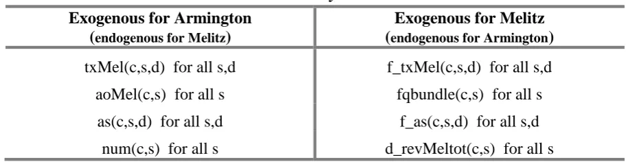
Table 1 shows the closure swaps required with our GTAP-A2M to move between Armington and Melitz specifications for industry c.
9
Table 1. Closure swaps for moving between Armington and Melitz specifications for industry c
Exogenous for Armington (endogenous for Melitz)
Exogenous for Melitz (endogenous for Armington)
txMel(c,s,d) for all s,d f_txMel(c,s,d) for all s,d
aoMel(c,s) for all s fqbundle(c,s) for all s
as(c,s,d) for all s,d f_as(c,s,d) for all s,d
num(c,s) for all s d_revMeltot(c,s) for all s
3. GTAP-A2M: illustrative Armington-Melitz comparison
This section compares two GTAP-A2M simulations of the effects of a 10 per cent increase (from 1.0989 to 1.2088) in the power of the North American (NAmerica) tariff on imports of Wearing apparel (wap). In the first simulation all industries are treated as Armington. In the second, the wap industry is Melitz while all others remain Armington. The switch from Armington to Melitz for the wap industry as we moved from the first simulation to the second was implemented by the closure swaps in Table 1.
We conducted the simulations in a 10-region, 57-commodity version of GTAP-A2M using GEMPACK software10. In both simulations we assumed that an increase in the NAmerica wap tariff has no effect on the balance of trade, investment and public consumption in any region. These are convenient simplifying assumptions. They allow us to measure welfare effects by the percentage changes in private consumption. For the wap industry under Melitz, we set the Pareto shape parameter () at 2 and the substitution elasticity between varieties () at 2.5. For the wap industry under Armington, the shape parameter plays no role. For the wap substitution elasticity in Armington we used the value 9.5 for both domestic/import and import/import substitution. Why 9.5? As we have argued elsewhere (Dixon et al., 2016), Armington-Melitz comparisons are facilitated by parameter choices that imply similar levels under the two specifications for the sensitivity of trade flows to tariff changes. We chose the Melitz and Armington values so that the effect on NAmerican wap imports of the 10 per cent tariff was the same in both simulations. With the values at 2.5 and 9.5, both simulations gave a 44 per cent reduction in the quantity of NAmerica’s wap imports.11
Figure 1 shows the regional welfare effects of the NAmerican wap tariff under Armington and Melitz specifications. As can be seen from the figure, under either specification SE Asia and South Asia are the main losers and NAmerica is the main winner. These qualitative results are unsurprising. SE Asia and South Asia have the biggest dependence of all the regions on exports of wap to NAmerica. For SE Asia the value of these exports in the GTAP database is 2.47 per cent of the total value of SE Asia’s private consumption (welfare). The corresponding percentage for South Asia is 1.20. In a simulation in which NAmerica makes a modest tariff increase from a low rate (9.89 per cent) without retaliation, we would expect it to derive a welfare gain via the optimal-tariff argument.
10 See Harrison et al. (2014) and Horridge et al. (2013).
10
Figure 1. A 10 per cent increase in the power of the Wap tariff on North American imports: welfare effects in Armington and Melitz
While Figure 1 shows the same winners and losers for Armington and Melitz, the Melitz results are generally more extreme: under Melitz the losers lose more and the winners gain more. In the remainder of this section we focus on the differences between the Armington and Melitz results for SE Asia, South Asia and NAmerica.
3.1. Decomposing the Armington and Melitz welfare effects
The GEMPACK code for GTAP-A2M includes a welfare decomposition that can be used in explaining differences between Armington and Melitz results. The decomposition identifies for each region the contributions to welfare of changes in:
(a) employment;
(b) efficiency in producing quality-adjusted units (scale effects);
(c) terms of trade (quality-adjusted prices of exports relative to those of imports); and (d) tax-carrying flows.
The algebraic specification of these contributions is set out in DJR (2018, section 7.4). Here we explain the nature of the four decomposition components by reference to Table 2 which shows the decomposition results for the three focus regions in our two simulations.
Contribution (a) is the percentage change in a region’s consumption made possible by
changes in output generated by changes in employment. In both simulations we assume there is no change in employment in any region.
Contribution (b) is the percentage change in a region’s consumption made possible by changes in output of quality-adjusted units per bundle of inputs. An example is the easiest way to explain what we mean by quality-adjusted units. If there is a 10 per cent increase in
-0.90 -0.80 -0.70 -0.60 -0.50 -0.40 -0.30 -0.20 -0.10 0.00 0.10 0.20
1 Oceania 2 EastAsia 3 SEAsia 4 SouthAsia 5 NAmerica 6 LatinAmer 7 EU_25 8 MENA 9 SSA 10 RoW
11
Table 2. Decomposition of the welfare effects of a 10 per cent tariff imposed by NAmerica on imports of Wearing apparel (wap)
Contributions from:
Welfare (%change) (a) Employment (b) Efficiency (c) Terms of trade (d) Tax-carrying flows Armington assumptions for all industries
SEAsia -0.34 0.00 0.00 -0.29 -0.05
SouthAsia -0.14 0.00 0.00 -0.10 -0.05
NAmerica 0.02 0.00 0.00 0.06 -0.04
Melitz assumptions for wap, Armington for all other industries
SEAsia -0.79 0.00 -0.89 0.17 -0.08
SouthAsia -0.39 0.00 -0.57 0.26 -0.08
NAmerica 0.10 0.00 0.16 -0.02 -0.04
Table 3. Percentage welfare effects of a 10% tariff imposed by NAmerica on imports of Wearing apparel (wap): decomposition of welfare differences between Melitz and Armington
Armington Melitz Difference Explained difference
Domestic supply cost
Rebalancing terms of trade
Other tax-carrying flows
(1) (2) (3) =(2) – (1) (4) =(5)+(6)+(7) (5) (6) (7)
SEAsia -0.34 -0.79 -0.45 -0.44 -0.26 -0.15 -0.03
SouthAsia -0.14 -0.39 -0.25 -0.21 -0.08 -0.10 -0.03
12
the number of cars sent from s to d [qs(cars,s,d)=10] and the suitability of these cars for satisfying the needs of users in d increases by 5 per cent [as(cars,s,d)= 5], then the quality-adjusted flow from s to d increases by 15.5 per cent [ =100*((1+10/100)*(1+5/100)-1)]. If at the same time the price per car sent from s to d increases by 8 per cent, then the price per quality-adjusted car increases by 2.86 per cent [=100*((1+8/100)/(1+5/100)-1)].
For Armington industries, GTAP-A2M specifies constant returns to scale (no fixed costs). For these industries, there are no changes in the quality of output [as(c,s,d) = 0 for all d]. Consequently in our first simulation in which all industries are Armington, inputs move in line with output, generating zero efficiency contributions in the Armington column (b) of Table 2. By contrast, the Melitz column (b) of Table 2 shows negative efficiency
contributions for SE Asia and South Asia and a positive contribution for NAmerica.
In quality-adjusted terms, Melitz industries exhibit increasing returns to scale. Industry c in region s can generate a 10 per cent increase in its quality-adjusted output defined by
quality d
q (c, s)
SMV(c, s, d) * qs(c, s, d) as(c, s, d) , (14)with less than a 10 per cent increase in input bundles [qquality(c,s) qbundle(c,s) 0]. It can
do this by exploiting economies of scale at either the firm level or industry level.
Consider firm-level economies of scale. If each existing c-firm in country s increases its sales on each link by 10 per cent [and there is no change of numbers of firms or numbers on links, num(c,s) =0 and numl(c,s,d) =0 for all d] then quality adjusted output at the industry level increases by 10 per cent. In this case there is no quality change [as(c,s,d)= 0 for all d, see equation (6)] but each firm (and hence the industry) increases its number of input bundles by less than 10 per cent [qbundle(c,s) <10]. This is because existing firms do not need to incur additional costs either to start business or to set up on links.
Alternatively, economies of scale could be achieved at the industry level, but not at the firm level. This would happen if each existing firm stayed unaltered, producing an unchanged amount for each link, while the increase in quality-adjusted output was achieved by expanding the number of firms. For example, if (c) = 2.5, then a 10 per cent increase in quality-adjusted output for the industry would be generated by a 6 per cent increase in the number of firms and the number on each link with no change in the sales of typical firms. The increase of 6 per cent in the number of firms on each link would generate a count increase [qs(c,s,d)] of 6 per cent and a quality increase of 4 per cent [as(c,s,d) =
numl(c,s,d)/(-1) = 6/1.5=4]. At the same time, with a 6 per cent increase in the number of firms that effectively duplicate existing firms, the increase in input bundles required by the industry would be 6 per cent.
In our experience with Melitz-based models, economies of scale at the industry level are generally more important than those at the firm level. As demonstrated in DJR (2018, Appendix 7.2), if input requirements for establishing a (c,s) firm and setting up on all trading links are constant [hf(c,s) = 0 and ff(c,s,d) = 0 for all d] then, at least in a simplified model, the average size of (c,s) firms is constant implying that on average there are no realized firm-level economies of scale.
13
Contribution (c) is the percentage change in a region’s consumption made possible by changes in the fob price of its exports relative to the cif price of its imports. In calculating terms-of-trade effects we continue to use quality-adjusted units.
With wap specified as an Armington industry, Table 2 shows negative terms-of-trade contributions for SE Asia and South Asia and a positive contribution for NAmerica. The NAmerica tariff reduces SE Asia’s and South Asia’s wap exports to NAmerica. Under our assumption of no change in trade balances, SE Asia and South Asia experience rebalancing real devaluation. These real-exchange-rate movements reduce SE Asia’s and South Asia’s imports and stimulate their exports (including wap). The reduction in SE Asia’s and South Asia’s imports barely affects foreign-currency supply prices to these regions: SE Asia’s and South Asia’s imports are generally only moderate fractions of other countries’ exports. On the other hand, under the Armington assumption that each country produces a distinctive version of each product, stimulation of demand for SE Asia’s and South Asia’s products requires reduction in their foreign-currency prices. This generates reductions in the terms of trade for the two regions. For NAmerica, the opposite argument applies. NAmerica’s wap imports fall. Rebalancing takes place via real appreciation which reduces in NAmerica’s exports with corresponding increases in their foreign-currency prices.
With wap specified as a Melitz industry, Table 2 gives positive rather than negative terms-of-trade contributions for SE Asia and South Asia and a negative rather than a positive
contribution for NAmerica. The rebalancing argument from the last paragraph continues to apply. However it is outweighed by Melitz effects on quality-adjusted wap prices. The contraction in wap output in SE Asia and South Asia and the consequent loss of efficiency causes an increase in wap supply prices of quality-adjusted units from these regions. This is sufficient to generate terms-of-trade improvements despite trade rebalancing via real
devaluation. For NAmerica, the negative terms-of-trade contribution under Melitz arises partly from reductions in the quality-adjusted prices of its wap exports. But this is a
negligible effect: NAmerica’s wap exports are small. The main reason that the terms-of-trade contribution to NAmerican welfare switches from positive to negative as we go from
Armington to Melitz is that NAmerica pays higher prices for quality-adjusted units of wap imports. Under Melitz (but not Armington), NAmerica’s tariffs reduce the ability of SE Asia and South Asia to supply cheap units of quality-adjusted wap.
Contribution (d) is the percentage increase (decrease) in consumption made possible by the expansion (contraction) of taxed flows. These expansions (contractions) raise (lower) welfare by raising (lowering) the use of commodities that the user values at the tax-inclusive price whereas the cost of providing them is valued at the tax-exclusive price. For SE Asia and South Asia, the negative tax-carrying flow contributions shown in Table 2 (-0.05 under Armington and -0.08 under Melitz for both regions) simply reflect reductions in
consumption: in both regions sales to households carry substantial indirect taxes. Thus, contribution (d) is not an explaining factor for the negative outcomes for SE Asian and South Asian consumption. Rather, it is a reinforcing factor, exacerbating negative outcomes caused by other factors.
In our tariff-increase experiments, the only significant component in contribution (d) for NAmerica arises from the contraction its imports of wap. As mentioned earlier this
14
Figure 2. North American imports of Wap
differences between the two simulations in changes in NAmerica’s tax-carrying flows, apart from wap imports.
3.2. Towards a fundamental explanation of the difference between Armington and Melitz welfare effects
Moving up and down the columns of Table 2 tells us a lot about how Armington and Melitz models operate. It tells us: that Melitz produces efficiency effects but Armington doesn’t; that Melitz terms-of-trade effects can be in the opposite direction to those in Armington; and that contributions from tax-carrying flows are broadly similar between the two models. However moving along the rows doesn’t give us a satisfying explanation of the net
differences between Armington and Melitz welfare effects. It doesn’t tell us what to expect from addition along any given row. All we can see is that the welfare results for SE Asia and South Asia are more negative under Melitz than Armington because the negative Melitz efficiency contributions for these regions outweigh the positive differences between the Melitz and Armington terms-of-trade contributions. For NAmerica, Table 2 tells us that the welfare effect is more favorable with Melitz than Armington because the positive Melitz efficiency contribution outweighs the negative difference between the Melitz and Armington terms-of-trade contribution.
In Table 3 we work towards a more fundamental explanation of the differences in our simulations between the Armington and Melitz welfare results. The main insight is that efficiency losses in SE Asia and South Asia reduce the welfare of these regions only through their effects on the cost of supplying quality-adjusted wap to domestic households. From a welfare point of view, the increase in the cost of supplying exports is offset by higher prices paid by foreigners. In Table 2, the Melitz efficiency contributions for SE Asia and South Asia cover the whole of the losses of wap efficiency while the Melitz terms-of-trade contributions include the offsetting higher wap export prices. To move toward a more
fundamental understanding of welfare differences between Melitz and Armington, we need to eliminate the offsetting overlap between the efficiency and terms of trade contributions.
1.0000 1.0989
0.6 0.33
Tariff- inclusive price
Quantity of imports, quality-adjusted: value at initial prices as per cent of total private consumption
Area = 0.042
1.2088
15
Referring to detailed results not shown in this paper, we find under Melitz assumptions that the NAmerican tariff causes increases of 13.07 per cent and 14.62 per cent in the cost to SE Asian and South Asian households of quality-adjusted units of domestic wap. These cost increases reflect output contraction with associated loss of scale economies. In the two regions domestic wap accounts for 1.99 and 0.54 per cent of aggregate consumption. Thus, the cost increases in supplying domestic wap generate welfare losses for the two regions of 0.26 per cent (= 0.0199*13.07) and 0.08 per cent (= 0.0054*14.62). These are welfare losses under Melitz that do not occur under Armington. They are entered in column (5) of Table 3 as explanators of the difference between Melitz and Armington welfare results.
For NAmerica, efficiency gains under Melitz reduce the cost to households of quality-adjusted units of domestic wap by 13.57 per cent. For these households, domestic wap accounts for 1.175 per cent of aggregate consumption. Thus, as shown in column (5) of Table 3, the cost reduction under Melitz in supplying domestic wap generates a 0.16 per cent increase in NAmerican welfare (= 0.01175*13.57).
In generating the entries for SE Asia and South Asia in column (6) of Table 3 we considered the terms-of-trade effects for these regions of rebalancing their trade to compensate for their losses of wap export revenue. As indicated by the extent of real devaluation, the rebalancing task is considerably more onerous under Melitz than under Armington. Real devaluation for SE Asia, measured by the reduction in its factor price index relative to the world price level, is 52 per cent greater under Melitz than under Armington. For South Asia, real devaluation is 104 per cent greater under Melitz than under Armington. Melitz requires extra real
devaluation because NAmerica’s tariffs are considerably more damaging to SE Asia’s and South Asia’s wap exports under Melitz than under Armington. Under Melitz, increased costs reduce the ability of SE Asia and South Asia to export wap to third markets. By contrast, under Armington real devaluation allows SE Asia and South Asia to increase their wap exports to third markets. As can be seen in Table 2, under Armington assumptions the terms-of-trade contributions for SE Asia and South Asia are -0.29 and -0.10 per cent. On the basis of the extra real devaluations (and extra stimulation of non-wap exports) required under
Melitz relative to Armington, we estimate that Melitz imposes extra rebalancing trade-of-trade losses for the two regions of 0.15 per cent (= 0.52*0.29) and 0.10 per cent (=1.04*0.10). These are the numbers shown for SE Asia and South Asia in column (6) of Table 3.
In generating the entry for NAmerica in column (6) of Table 3 we considered the terms-of-trade effect for this region of rebalancing its terms-of-trade to compensate for the gain in its wap export revenue. This parallels the approach we used for the other two regions. But for NAmerica the change in wap export revenue is negligible. Consequently, for NAmerica we can ignore the interaction between wap efficiency and the terms of trade. Thus, for this region we show in column (6) of Table 3 the whole of the difference between the Melitz and Armington terms-of-trade results from column (c) in Table 2.
16
3.3. Summing up
Comparison of columns (3) and (4) in Table 3 indicates that our back-of-the-envelope calculations for the three effects in columns (5), (6) and (7) do not provide a completely accurate decomposition of the difference between the Melitz and Armington welfare effects in our two simulations. Nevertheless they tell most of the story.
They tells us that the principal losers, SE Asia and South Asia, lose more welfare under Melitz than under Armington for two reasons. First, Melitz recognizes that the contraction of SE Asia’s and South Asia’s wap industries generates an increase in the cost to households in these two regions of domestically-supplied wap products. This welfare-reducing effect is not present in Armington. Second, the NAmerican tariff does more damage to SE Asia’s and South Asia’s wap industries under Melitz than under Armington, even when we normalize so that the contraction in exports from these regions to NAmerica is the same under both sets of assumptions. This is because in Melitz (but not in Armington) cost increases in SE Asia’s and South Asia’s wap industries caused by loss of scale economies reduce the two regions’ wap export revenue from third markets. Consequently, greater stimulation of SE Asia’s and South Asia’s non-wap exports is required under Melitz than under Armington. Greater stimulation of these non-wap exports causes a larger welfare-reducing terms-of-trade reduction.
For NAmerica, the story from column (5) of Table 3 is that welfare under Melitz (but not Armington) is increased by the expansion of the domestic wap industry which reduces the cost to NAmerican households of domestically-produced wap. On the other hand, welfare under Melitz (but not Armington) is reduced by increases in the cost to NAmerica of
imported wap caused by loss of scale economies in supplying regions. This effect is reflected in the negative entry in column (6) of Table 3. A priori it was not clear that the positive entry for NAmerica in column (5) would outweigh the negative entry in column (6). The balance depends on the data. For example, if we considered a situation in which the domestic/import wap ratio in the NAmerican market is smaller than that in the GTAP database, then we might find that the negative entry in column (6) outweighs the positive entry in column (5).
4. Relationship between GTAP-HET and GTAP-A2M
In creating the GTAP-A2M system our main objective was to give users of the GTAP model the option of switching from Armington to Melitz for industries of their choice. This was also the objective of AVH (2016) in creating GTAP-HET.12
What are the advantages and disadvantages of GTAP-HET versus GTAP-A2M? The
advantage of GTAP-HET is that it allows for the composition of inputs to current production in an industry to be different from that used in establishing firms and setting up on trade links. In GTAP-A2M we assume no difference between the composition of input bundles used by industry (c,s) in current production from that of bundles used in meeting fixed-cost requirements. In the 2016 version of GTAP-HET this advantage hadn’t been pushed very far. It was assumed that all fixed cost requirements in industry (c,s) are met with input-bundles consisting entirely of primary factors with the same mix and substitution possibilities as the primary factors used by (c,s) in current production. In Akgul et al. (2017) a serious effort was made to identify the occupational composition of the labor input to fixed costs. Work along these lines has the potential to make GTAP-HET’s distinction between current and fixed input composition worthwhile. However, a disadvantage of the distinction is that it requires extensive changes in GTAP’s input demand equations to separate demands for inputs
17
to current production from demands for inputs to fixed costs.13 By contrast, GTAP-A2M leaves the original GTAP model almost untouched. We simply add some rather trivial equations on the end and implement them with closure swaps.
As demonstrated in DJR (2018, Appendix 7.3), a problem with GTAP-HET is that it fails to incorporate Melitz pricing to market. Instead of equation (5), in the notation of this paper GTAP-HET specifies that Melitz industries price according to
ave
(c) 1
pmarket(c,s, d) pbundle(c,s) ptivity (c,s) (c)
(14)
Notice that there is no d argument on the right hand side of (14). The same market price applies to all destinations. In (14) GTAP-HET changes (5) by replacing the percentage change in the marginal productivity of the typical c-firm on the s,d-link with the percentage change in marginal productivity averaged over all (c,s) firms. The coefficient
( (c) 1) / (c) is the share of variable costs in (c,s)’s total costs. Its inclusion on the right hand side of (14) is intended to capture the idea that changes in marginal productivity operate on variable costs, not total costs.
Equation (14) is inconsistent with Melitz theory. AVH do not produce any other theory to justify it. In our view, (14) is a mistake. But does it matter? Simulations with a stylized model reported in DJR (2018) suggest that the answer is yes. In any case, inclusion of (14) along with a tortuous but ad hoc definition of ptivityave(c,s) certainly impede understanding of GTAP-HET and interpretation of its results.
5. Concluding remarks
The GTAP-A2M system makes it possible for users of the GTAP model to explore the implications of Melitz theory in a computing system with which they are familiar. There are no new data requirements, beyond assigning values for the Pareto shape parameter () and revising the Armington substitution elasticities () so that they take on values suitable for substitution elasticities between varieties rather than countries. There are no new
dimensional limitations. In the GTAP-A2M system computed with GEMPACK, an r-region, n-industry model incorporating Melitz industries takes barely any longer to solve than if all the industries were Armington.
In our earlier paper in this journal, Dixon et al. (2016), we sided cautiously with Arkolakis et al. (2012)’s “same-old-gains” paper which argues on the basis of theory that welfare results from Melitz models are unlikely to be much different from those of Armington models. Our opinion was coloured by results from a stylized numerical model in which we inadvertently adopted simplifying assumptions similar to those in Arkolakis et al.’s basic theoretical model.
Our assumptions included: (a) one factor of production in each region; (b) no intermediate inputs; (c) all industries being either Melitz or Armington; and (d) the same parameter values in each industry. The basic theoretical model of Arkolakis et al. explicitly adopts (a) and (b). Because Arkolakis et al. allowed for only one industry in each region, they implicitly adopted (c) and (d). Not surprisingly, the numerical results from Dixon et al. (2016) supported the theoretical results from Arkolakis et al. (2012).
What we found from the GTAP-A2M system is that conclusions derived in a model
embracing (a) to (d) are not readily generalizable. If some industries are modelled as Melitz
13 AVH also introduce explicit modifications to standard GTAP to eliminate the two-tier import/domestic
18
and others as Armington, then the simulated welfare effects of trade policies can be quite different from those obtained when all industries are Armington. In our simulations of a tariff increase by NAmerica on wap imports, we compared GTAP-A2M results in which wap was modelled as Melitz and all other industries were Armington with results in which all industries were Armington. In these simulations, resources in SE Asia and South Asia are transferred out of wap and into other industries, while the opposite happens for NAmerica. We found that when wap was treated as a Melitz industry (with increasing-returns-to-scale) the transfer of resources in SE Asia and South Asia into Armington industries (with constant returns to scale) generated significant additional welfare losses for these regions compared with the situation in which all industries were Armington. Similarly, expansion of the wap industry in NAmerica generated an additional welfare gain for NAmerica when wap was Melitz that was not present when wap was Armington.
Armington has been the workhorse trade specification in CGE modelling since the 1970s. 14 Should it be replaced by mixed-Armington-Melitz specifications? We hope that the GTAP-A2M system facilitates the research necessary to continue teasing out the implications of Melitz assumptions and the realism of the results. One final hint. In understanding Melitz results via explanatory back-of-the-envelope calculations, it is helpful to work with quality-adjusted prices and quantities. Working with these concepts allows us to think in terms of stable demand and supply diagrams.
References
Akgul, Z., N.B. Villoria and T.W. Hertel (2016), “GTAP-HET: Introducing Firm
Heterogeneity into the GTAP Model”, Journal of Global Economic Analysis, vol. 1(1), pp. 111-180.
Akgul, Z., C. Carrico and M. Tsigas (2017), “Does the labor composition of fixed business costs matter?”. Paper presented at the 20th Annual GTAP Conference, held at Purdue University, West Lafayette, Indiana, June, pp. 19.
Arkolakis, C., A. Costinot, A. Rodriguez-Clare (2012), “New trade models, same old gains?”,
American Economic Review, 102(1), pp. 94-130.
Armington, P. (1969), “A theory of demand for products distinguished by place of production”, Staff Papers-International Monetary Fund,16(1), 159–178.
Corong, E., T. Hertel, R. McDougall, M. Tsigas and D. van der Mensbrugghe (2017), “The standard GTAP model, Version 7”, Journal of Global Economic Analysis,vol. 2(1), pp. 1-119.
Deardorff, A.V., R.M. Stern and C.F. Baum (1977), “A multi-country simulation of the employment and exchange-rate effects of post-Kennedy round tariff reductions” , Chapter 3, pp. 36-72 in N. Akrasanee, S. Naya and V.Vichit-Vadakan (editors), Trade and Employment in Asia and the Pacific, the University Press of Hawaii, Honolulu. Dixon, P.B., B.R. Parmenter, G.J. Ryland and J. Sutton (1977), ORANI, AGeneral
Equilibrium Model of the Australian Economy: CurrentSpecification and Illustrations of Use for Policy Analysis, Vol. 2 of the First Progress Report of the IMPACT Project, Australian Government Publishing Service, Canberra, pp. xii + 297.
Dixon, P.B., B.R. Parmenter, John Sutton and D.P. Vincent (1982), ORANI: A Multisectoral Model of the Australian Economy, Contributions to Economic Analysis 142, North-Holland Publishing Company, pp. xviii + 372.
19
Dixon, P.B., M. Jerie and M.T. Rimmer (2016), “Modern Trade Theory for CGE Modelling: the Armington, Krugman and Melitz Models”, Journal of Global Economic Analysis, vol. 1(1), pp. 1-110.
Dixon, P.B., M. Jerie and M.T. Rimmer (2018), Trade theory in computable general equilibrium models: Armington, Krugman and Melitz, Advances in Applied General Equilibrium Modelling, Springer Nature, Singapore, pp. xi + 189
Harrison, J., J.M. Horridge, M. Jerie and K.R. Pearson (2014), GEMPACK manual, GEMPACK Software, ISBN 978-1-921654-34-3, available at
http://www.copsmodels.com/gpmanual.htm .
Hertel, T. W., editor, (1997), Global trade analysis: modeling and applications, Cambridge University Press, Cambridge, UK.
Horridge, M., A Meeraus, K. Pearson and T. Rutherford (2013), “Software platforms: GAMS and GEMPACK”, chapter 20, pp. 1331-82, in P.B. Dixon and D.W. Jorgenson (editors)
Handbook of Computable General Equilibrium Modeling, Elsevier, Amsterdam. Melitz, Marc J. (2003), “The impact of trade on intra-industry reallocations and aggregate