The TERM model and its data base

(1)

Eleventh Floor, Menzies Building Monash University, Wellington Road CLAYTON Vic 3800 AUSTRALIA

from overseas: Telephone:

(03) 9905 2398, (03) 9905 5112 61 3 9905 2398 or

61 3 9905 5112 Fax:

(03) 9905 2426 61 3 9905 2426

e-mail: [email protected]

Internet home page: http//www.monash.edu.au/policy/

The TERM model and its data base

by

M

ark

HORRIDGE

Centre of Policy Studies, Monash University

General Paper No. G-219 July 2011

ISSN 1 031 9034 ISBN 978 1 921654 26 8

(2)

by Mark Horridge,

Centre of Policy Studies, Monash University, Australia

Draft chapter for forthcoming book published by Springer:

"Economic Modelling of Water: The Australian CGE Experience", edited by Glyn Wittwer.

Abstract

TERM (The Enormous Regional Model) provides a strategy for creating a "bottom-up" multi-regional CGE model which treats each region of a single country as a separate economy. This makes it a useful tool for examining the regional impacts of shocks that may be region-specific. TERM is designed to allow quick simulations with many regions, so allowing for models of large countries with 30 to 50 provinces, such as USA or China. TERM also offers a standard procedure for preparing a database which requires, in addition to a national input-output or use-supply table, a minimal amount of regional data. More regional data can be used if available.

JEL classification: C68, D58, R12, R13 Keywords: Regional CGE

5.1. The false allure of regional input-output tables 10 5.2. The TERM data strategy 11 5.3. The national input-out database 12 5.4. Estimates of the regional distribution of output and final demands 12 5.5. The TRADE matrix 13 5.6. Aggregation 15 6. Conclusion: applications and developments of TERM... 18

Tables

Table 1: Main sets of the TERM model... 3

Figures

Figure 1: The TERM flows database ... 5

Figure 2: TERM production structure...7

Figure 3: TERM sourcing mechanisms ...9

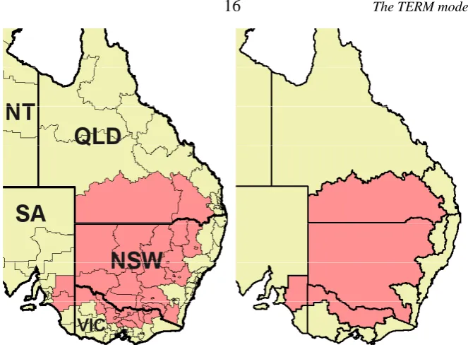
Figure 4: Statistical divisions in Australia ... 15

Figure 5: Aggregating from master database to policy simulation (watershed) regions ...16

(3)

The TERM model and its data base

1

by Mark Horridge

Centre of Policy Studies, Monash University, Australia

1. Introduction

TERM is a framework for CGE (computable general equilibrium) modelling of multiple regions within a single country. It was developed to address two common problems of multi-regional CGE models:

• as the number of regions increases, simulations became very slow, or require large amounts of memory.

• it is difficult to develop a database for such models; published data is usually quite sparse. TERM offers a solution to both problems:

• the database and equation system are structured to allow fast solutions with small memory needs. An inbuilt automatic system to aggregate regions and/or sectors allows model size to be reduced to speed simulations, while preserving detail that is needed for a particular application.

• there is a standard procedure for preparing a database which requires, in addition to a national input-output or use-supply table, a minimal amount of regional data. More regional data can be used if available.

From the outset the TERM framework has been intended as a template which might be quickly ap-plied to a variety of countries. Thus the standard version of TERM is fairly simple, avoiding mechanisms which might be specific to a particular country or application. Rather the emphasis is on allowing a basic multi-regional model to produce simulation results as soon as possible. Very often, analysis of results reveals shortcomings of the model or data , or suggests priorities for im-provement. To arrive quickly at this stage is key to the quality of the final model.

TERM builds on the ORANI model (Dixon et al., 1982), which distinguished over 100 sectors, and introduced large-scale computable general equilibrium modelling in 1977. In particular, the minimal data requirements for constructing a TERM database scarcely exceed those for a "top-down" multi-regional version of ORANI, described below. In fact, the standard procedure for pre-paring a TERM assumes that a working "topdown" database has already been prepared and used for simulations. This allows most potential problems with regional data to be noticed and fixed at an early stage.

2. Progress in Australian regional economic modelling

Since ORANI, related models have developed in several new directions. ORANI's solution algo-rithm combined the efficiency of linearised algebra with the accuracy of multi-step solutions, al-lowing the development of ever more disaggregated and elaborate models. The GEMPACK soft-ware developed by Ken Pearson (1988) and colleagues since the mid-1980s simplified the specifi-cation of new models, while cheaper, more powerful computers allowed the development of com-puter-intensive multi-regional and dynamic models.

On the demand side, these advances have been driven by the appetite of policy-makers for sec-toral, regional, temporal, and social detail in analyses of the effects of policy or external shocks. Since parliamentary representatives are elected by regions, demand for regional detail is particularly strong.

To meet this need, even early versions of ORANI (see Dixon et al. 1978) included a “top-down” regional module to work out the regional consequences of national economic changes: na-tional results for quantity (but not price) variables were broken down by region using techniques

1

(4)

borrowed from input-output analysis. The name "top-down" reflects the feature that national results drive regional results and are unaffected by the regional subsystem. Key assumptions are:

• for each sector the technology of production (ie, cost shares) is uniform across regions.

• for commodities that are heavily traded between regions (the "national" commodities), each re-gion's share of national output is fixed or exogenous. So for these sectors, the percent change in output is uniform across regions.

• for the remaining, "local", commodities (that are little traded between regions) output in each region adjusts to meet demand in that region.

Using the top-down technique, from 8 to 100 regions can easily be distinguished. Region-specific demand shocks may be simulated, but, since price variables have no regional dimension, there is little scope for region-specific supply shocks2. On the other hand, the “top-down” approach requires little extra data or computer power.

A second generation of regional CGE models adapted ORANI by adding two regional sub-scripts (source and destination) to many variables and equations. In this “bottom-up” type of multi-regional CGE model, national results are driven by (ie, are additions of) multi-regional results. Liew (1984), Madden (1989) and Peter et al.(1996) describe several Australian examples. Dynamic ver-sions of such models have followed (Giesecke 1997). The best-known example of this type of re-gional model is the Monash Multirere-gional Forecasting model, MMRF (Adams et al. 2002).

Bottom-up models allow simulations of policies that have region-specific price effects, such as a payroll tax increase in one region only. They also allow us to model imperfect factor mobility (between regions as well as sectors). Thus, increased labour demand in one region may be both choked off by a local wage rise and accommodated by migration from other regions. Unfortunately models like MMRF pose formidable data and computational problems—limiting the amount of sectoral and regional detail. Only 2 to 8 regions and up to 40 sectors could be distinguished3. Luck-ily, Australia has only 8 states, but size limitations have hindered the application of similar models to larger countries with 30 to 50 provinces, and have hitherto prevented us from distinguishing smaller, sub-state regions.

Finer regional divisions are desirable for several reasons. Policy-makers who are concerned about areas of high unemployment or about disparities between urban and rural areas desire more detailed regional results. Environmental issues, such as water management, often call for smaller regions that can map watershed or other natural boundaries more closely. Finally, more and smaller regions give CGE models a greater sense of geographical realism, closing the gap between CGE and LUTE (Land Use Transportation Energy) modelling.

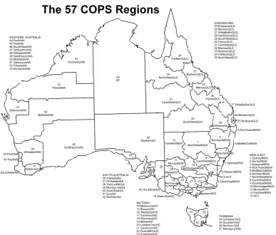
The TERM4 model adds to the ORANI/MMRF tradition by allowing greater disaggregation of regional economies than was previously available. For example, it allows us to analyse effects for each of 57 statistical divisions within Australia—which would be computationally infeasible using the MMRF framework.

3. The structure of TERM

A key feature of TERM, in comparison to predecessors such as MMRF, is its ability to handle a greater number of regions or sectors. The greater efficiency arises from a more compact data struc-ture, made possible by a number of simplifying assumptions.

3.1. Defeating the curse of dimensionality

The database for a CGE model consists of matrices of flow values dimensioned by commodity, in-dustry and region. The model will contain quantity and price variables for each of these flows, so the number of variables and equations tends to track database size. The computer resources (time

2

Such limitations could be partially circumvented: see Higgs et al., 1988. 3

More precisely, these 2nd-generation models (like MMRF) become rather large and slow to solve as the product: (number of regions) x (number of sectors) exceeds 300. TERM raises this limit to about 2500.

4

(5)

and memory) needed to solve the model increase super-proportionately5 as the size of the database increases. Indeed a doubling of database size may multiply solution time by 3. Sectoral or regional detail may have to be sacrificed to reduce computing problems.

To illustrate, the value of intermediate demands in a single-region CGE model (like ORANI) might be represented by a matrix V, with dimensions COM*IND, where, for example:

V("Coal","Steel") = value of Coal used by the Steel industry. With 50 commodities and industries, V would contain 2500 elements.

In the MMRF framework, V would be dimensioned COM*IND*REG*REG, where the first regional subscript denotes the region of origin of some input, and the second regional subscript de-notes the region where the input is used. Since MMRF distinguishes 8 Australian states, the V ma-trix would be 64 times bigger than in ORANI—leading to much larger (but just acceptable) solution times. A USA version of MMRF, distinguishing 50 states, would imply a database which was 70 [=(50/8)2] times larger than the 8-state MMRF, leading to model solution times and memory re-quirements perhaps 500 times those of the Australian MMRF—which is quite impractical.

TERM's solution to this problem is to restructure the model database so that no matrix contains more than 3 of the "large" COM, IND or REG dimensions. For example, instead of the large 4-dimensional intermediate input matrix used by MMRF: V(COM, IND, REG, REG), we could in-stead use two 3-dimensional matrices:

V(COM, IND, REG) = value of commodities used by industries in region of use; and T(COM, REG, REG) = value of commodities used, by regions of production and use.

which together are 25 times smaller (with 50 sectors and regions), leading to model solution times and memory requirements perhaps 125 times less. The cost is a small loss in generality: the sourcing or trade matrix T encapsulates the assumption that all users in a particular region of, say, vegetables, source their vegetables from other regions according to common proportions.

3.2. The TERM data structure

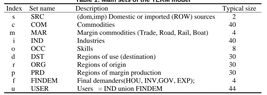
Figure 1 is a schematic representation of the model's input-output database. It reveals the basic structure of the model, which is key to its efficiency. The rectangles indicate matrices of flows. Core matrices (those stored on the database) are shown in bold type; the other matrices may be cal-culated from the core matrices. The dimensions of the matrices are indicated by indices (c, s, i, m, etc) which correspond to the following sets:

Table 1: Main sets of the TERM model

Index Set name Description Typical size

s SRC (dom,imp) Domestic or imported (ROW) sources 2

c COM Commodities 40

m MAR Margin commodities (Trade, Road, Rail, Boat) 4

i IND Industries 40

o OCC Skills 8

d DST Regions of use (destination) 30

r ORG Regions of origin 30

p PRD Regions of margin production 30

f FINDEM Final demanders(HOU, INV,GOV, EXP); 4

u USER Users = IND union FINDEM 44

The sets DST, ORG and PRD are in fact the same set, named according to the context of use. The matrices in Figure 1 show the value of flows valued according to 3 methods:

5

(6)

1) Basic values = Output prices (for domestically-produced goods), or CIF prices (for imports) 2) Delivered values = Basic + Margins

3) Purchasers' values = Basic + Margins + Tax = Delivered + Tax

The matrices on the left-hand side of the diagram resemble (for each region) a conventional single-region input-output database. For example, the matrix USE at top left shows the delivered value of demand for each good (c in COM) whether domestic or imported (s in SRC) in each desti-nation region (DST) for each user (USER, comprising the industries, IND, and 4 final demanders: households, investment, government, and exports). Some typical elements of USE might show:

USE("Wool","dom","Textiles","North") : domestically-produced wool used by the textile in-dustry in North

USE("Food","imp","HOU","West") : imported food used by households in West

USE("Meat","dom","EXP","North") : domestically-produced meat exported from a port in North. Some of this meat may have been produced in another region.

USE("Meat","imp","EXP","North") : imported meat re-exported from a port in North

As the last example shows, the data structure allows for re-exports (at least in principle). All these USE values are "delivered": they include the value of any trade or transport margins used to bring goods to the user. Notice also that the USE matrix contains no information about regional sourcing of goods.

The TAX matrix of commodity tax revenues contains an element corresponding to each ele-ment of USE. Together with matrices of primary factor costs and production taxes, these add to the costs of production (or value of output) of each regional industry.

In principle, each industry is capable of producing any good. The MAKE matrix at the bottom of Figure 1 shows the value of output of each commodity by each industry in each region. A subto-tal of MAKE, MAKE_I, shows the tosubto-tal production of each good (c in COM) in each region d.

TERM recognizes inventory changes in a limited way. First, changes in stocks of imports are ignored. For domestic output, stock changes are regarded as one destination for industry output (ie, they are dimension IND rather than COM). The rest of production goes to the MAKE matrix.

The right hand side of Figure 1 shows the regional sourcing mechanism. The key matrix is TRADE, which shows the value of inter-regional trade by sources (r in ORG) and destinations (d in DST) for each good (c in COM) whether domestic or imported (s in SRC). The diagonal of this matrix (r=d) shows the value of local usage which is sourced locally. For foreign goods (s="imp") the regional source subscript r (in ORG) denotes the port of entry. The matrix IMPORT, showing total entry of imports at each port, is simply an addup (over d in DST) of the imported part of TRADE.

The TRADMAR matrix shows, for each cell of the TRADE matrix the value of margin good m (m in MAR) which is required to facilitate that flow. Adding together the TRADE and TRADMAR matrix gives DELIVRD, the delivered (basic + margins) value of all flows of goods within and between regions. Note that TRADMAR makes no assumption about where a margin flow is pro-duced (the r subscript refers to the source of the underlying basic flow).

Matrix SUPPMAR shows where margins are produced (p in PRD). It lacks the good-specific subscripts c (COM) and s (SRC), indicating that, for all usage of margin good m used to transport any goods from region r to region d, the same proportion of m is produced in region p. Summation of SUPPMAR over the p (in PRD) subscript yields the matrix SUPPMAR_P which should be iden-tical to the subtotal of TRADMAR (over c in COM and S in SRC), TRADMAR_CS. In the model, TRADMAR_CS is a CES aggregation of SUPPMAR: margins (for a given good and route) are sourced according to the price of that margin in the various regions (p in PRD).

(7)

HOUPUR(c,h,d) purchasers value of good c used

by household type h in d price: phou(c,d) quantity: xhouh_s(c,h,d);

INVEST(c,i,d) purchasers value of good c used for investment in industry i in d

price: pinvest(c,d) quantity: xinvi(c,i,d);

USER x DST DST ORG x DST

COM x SRC IND USE (c,s,u,d) Delivered value of demands:

basic + margins (ex-tax) quantity: xint(c,s,i,d) price: puse(c,s,d) FINDEM (HOU,INV, GOV, EXP) quantities: xhou(c,s,d) xinv(c,s,d) xgov(c,s,d) xexp(c,s,d) final de-mands by 4

users at delivered price: puse(c,s,d) = USE_U (c,s,d) = DELIVRD_R (c,s,d) price: pdelivrd_r (c,s,d) quantity: xtrad_r (c,s,d) = CES DELIVRD (c,s,r,d) = TRADE(c,s,r,d)

+ sum{m,MAR, TRADMAR(c,s,m,r,d)} price: pdelivrd (c,s,r,d) quantity: xtrad(c,s,r,d)

+ = {Leontief)

COM x SRC TAX (c,s,u,d) Commodity taxes TRADE (c,s,r,d)

good c,s from r to d at basic prices quantity: xtrad(c,s,r,d) price: pbasic(c,s,r) IMPORT (c,r) + + FACTORS

LAB(i,o,d) wages

CAP(i,d) capital rentals

LND(i,d) land rentals

PRODTAX(i,d) production tax

MAKE_I(c,r) = TRADE_D (c,"dom",r) TRADMAR (c,s,m,r,d)

margin m on good c,s from r to d quantity: xtradmar(c,s,m,r,d)

price: psuppmar_p(m,r,d)

= sum over COM and SRC INDUSTRY OUTPUT:

VTOT(i,d) TRADMAR_CS(m,r,d)

= =

INVENTORIES: STOCKS(i,d) SUPPMAR_P(m,r,d) + CES sum over p in REGPRD

COM

MAKE

(c,i,d)

output of good c by industry I in d update: xmake(c,i,d)*pdom(c,d)

sum over i in IND =

MAKE_I (c,d) domestic commodity supplies SUPPMAR (m,r,d,p)

Margins supplied by p on goods passing from r to d update: xsuppmar(m,r,d,p)*pdom(m,p)

MAKE_I(m,p) = SUPPMAR_RD(m,p) + TRADE_D (m,"dom",p) IND x DST DST ORG x DST

Figure 1: The TERM flows database

Index Set Description

c COM Commodities

s SRC Domestic or imported (ROW) sources m MAR Margin commodities

r ORG Regions of origin d DST Regions of use (destination) p PRD Regions of margin production

f FINDEM Final demanders(HOU, INV,GOV, EXP) i IND Industries

u USER Users = IND union FINDEM o OCC Skills

(8)

A balancing requirement of the TERM database is that the sum over user of USE, USE_U, shall be equal to the sum over regional sources of the DELIVRD matrix, DELIVRD_R.

It remains to reconcile demand and supply for domestically-produced goods. In Figure 1 the connection is made by arrows linking the MAKE_I matrix with the TRADE and SUPPMAR matri-ces. For non-margin goods, the domestic part of the TRADE matrix must sum (over d in DST) to the corresponding element in the MAKE_I matrix of commodity supplies. For margin goods, we must take into account both the margins requirement SUPPMAR_RD and direct demands TRADE_D.

At the moment, TERM distinguishes only 4 final demanders in each region: (a) HOU: the representative household

(b) INV: capital formation (c) GOV: government demand (d) EXP: export demand.

For many purposes it is useful to break down investment according to destination industry. The sat-ellite matrix INVEST (subscripted c in COM, i in IND, and d in DST) serves this purpose. It allows us to distinguish the commodity composition of investment according to industry: for example, we would expect investment in agriculture to use more machinery (and less construction) than invest-ment in dwellings.

Similarly, another satellite matrix, HOUPUR, allows us to distinguish several household types with different budget shares. Both satellite matrices enforce the assumption that import/domestic shares and commodity tax rates are uniform across household (or investor) types: For example we assume that the tax rate on cigarettes is the same for rich and poor, as is the share of imports in ciga-rette consumption.

Missing from Figure 1 is an account of how factor incomes and tax revenue accrue to regional households and governments. Such data would be needed to convert the TERM data schema into a complete SAM. Australian versions of TERM typically assume that wage income generated in re-gion A accrues to households in rere-gion A, while capital income goes into a national "pot" which is shared between regional households. Similarly, tax revenue accrues to a national authority which distributes it between regions. Such assumptions might be inappropriate if TERM were applied to other countries. For example, in the USA some taxes accrue directly to state governments, and wage income generated in Washington DC may well be spent by households in Maryland or Virginia. Hence the generic version of TERM enforces no default system: users must devise their own map-ping of income to agents, appropriate to a particular country. Their decisions may be be influenced by the chosen level of regional detail. For example, some Australian versions of TERM distinguish 57 'statistical division' regions which do not entirely correspond with administrative regions -- so regional government incomes are not modelled in these versions.

4. The TERM equation system

(9)

KEY

Inputs or Outputs Functional

Form

CES CES Leontief

CES CES

up to Labour

type O Labour

type 2 Labour

type 1

Capital Labour

Land

Primary Factors

Imported Good G Domestic

Good G Imported

Good 1 Domestic

Good 1

Good G Good 1

CES 0.15 0.5

1.5

0.35 0

Intermedi ate

CET

up to Good G

Good 2 Good 1

Activity Level

0.5 _STOCKS

(10)

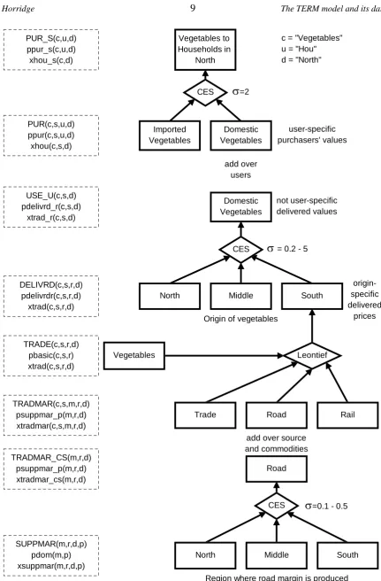
4.1. TERM sourcing mechanisms

Figure 3 illustrates the details of the TERM system of demand sourcing. Although the figure covers only the demand for a single commodity (Vegetables) by a single user (Households) in a single re-gion (North), the same diagram would apply to other commodities, users and rere-gions. The diagram depicts a series of 'nests' indicating the various substitution possibilities allowed by the model. Down the left side of the figure, boxes with dotted borders show in upper case the value flows asso-ciated with each level of the nesting system. These value flows may also be located in Figure 1. The same boxes show in lower case the price (p....) and quantity (x....) variables associated with each flow. The dimensions of these variables are critical both to the usefulness of the model and to its computational tractability; they are indicated by subscripts c, s, m, r, d and p, as explained in Table 1. Most of what is innovative in TERM could be reconstructed from Figures 1 and 2.

At the top level, households choose between imported (from another country) and domestic vegetables. A CES or Armington specification describes their choice—as pioneered by ORANI and adopted by most later CGE models. Demands are guided by user-specific purchasers' prices (the purchasers' values matrix PUR is found by summing the TAX and USE matrices of Figure 1). 2 is a typical value for the elasticity of substitution.

Demands for domestic vegetables in a region are summed (over users) to give total value USE_U (the "_U" suffix indicates summation over the user index u). The USE_U matrix is meas-ured in "delivered" values—which include basic values and margins (trade and transport), but not the user-specific commodity taxes.

Moving down, the next level treats the sourcing of USE_U between the various domestic re-gions. The matrix DELIVRD shows how USE_U is split between origin regions r. Again a CES specification controls the allocation; substitution elasticities range from 5 (merchandise) to 0.2 (services). The CES implies that regions which lower production costs more than other regions will tend to increase their market share. The sourcing decision is made on the basis of delivered prices— which include transport and other margin costs. Hence, even with growers' prices fixed, changes in transport costs will affect regional market shares. Notice that variables at this level lack a user (u) subscript—the decision is made on an all-user basis (as if wholesalers, not final users, decided where to source vegetables). The implication is that, in North, the proportion of vegetables which come from South is the same for households, intermediate, and all other users.

The next level down shows how a "delivered" vegetable from, say, South, is a Leontief com-posite of basic vegetable and the various margin goods. The share of each margin in the delivered price is specific to a particular combination of origin, destination, commodity and source. For ex-ample, we should expect transport costs to form a larger share for region pairs which are far apart, or for heavy or bulky goods. The number of margin goods will depend on how aggregated is the model database. Under the Leontief specification we preclude substitution between Road and Retail margins, as well as between Road and Rail. For some purposes it might be worthwhile to construct a more elaborate nesting which accommodated Road/Rail switching.

The bottom part of the nesting structure shows that margins on vegetables passing from South to North could be produced in different regions. The figure shows the sourcing mechanism for the road margin. We might expect this to be drawn more or less equally from the origin (South), the destination (North) and regions between (Middle). There would be some scope (σ=0.5) for substi-tution, since trucking firms can relocate depots to cheaper regions. For retail margins, on the other hand, a larger share would be drawn from the destination region, and scope for substitution would be less (σ=0.1). Once again, this substitution decision takes place at an aggregated level. The as-sumption is that the share of, say, Middle, in providing Road margins on trips from South to North, is the same whatever good is being transported.

(11)

North Middle South Vegetables

Trade Road Rail North Middle South

Vegetables to Households in

North

Domestic Vegetables Imported

Vegetables PUR_S(c,u,d)

ppur_s(c,u,d) xhou_s(c,d)

CES CES

Leontief

CES DELIVRD(c,s,r,d)

pdelivrdr(c,s,r,d) xtrad(c,s,r,d) PUR(c,s,u,d) ppur(c,s,u,d) xhou(c,s,d)

TRADE(c,s,r,d) pbasic(c,s,r) xtrad(c,s,r,d)

TRADMAR(c,s,m,r,d) psuppmar_p(m,r,d) xtradmar(c,s,m,r,d)

SUPPMAR(m,r,d,p) pdom(m,p) xsuppmar(m,r,d,p)

add over source and commodities

Region where road margin is produced Origin of vegetables

Domestic Vegetables

add over users

USE_U(c,s,d) pdelivrd_r(c,s,d)

xtrad_r(c,s,d)

user-specific purchasers' values

origin-specific delivered

prices not user-specific

delivered values c = "Vegetables" u = "Hou" d = "North"

Road TRADMAR_CS(m,r,d)

psuppmar_p(m,r,d) xtradmar_cs(m,r,d)

σ=0.1 - 0.5

σ=2

σ = 0.2 - 5

(12)

4.2. Other features of TERM

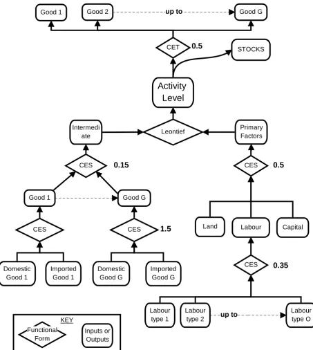
The remaining features of TERM are common to most CGE models, and in particular to ORANI, from which TERM descends. Industry production functions are of the nested CES type: Leontief except for substitution between primary factors and between sources of goods. Exports from each region's port to the ROW face a constant elasticity of demand. The composition of household de-mand follows the linear expenditure system, while the composition of investment and government demands is exogenous. A variety of closures are possible. For the shortrun simulation we might hold fixed industry capital stocks and land endowments, whilst allowing labour to be fully mobile between sectors within a region and partially mobile between regions. At the regional level we may link household consumption to regional factor incomes.

4.2.1. National and regional macro closures

Closure flexibility in TERM applies separately at the national and regional levels. For example, we may wish to impose a balance of trade constraint at the national level, without however enforcing balanced trade for each region. We might stipulate that regional consumption Cr follows wage

in-come Wr via a rule like:

Cr = FrWrλ

where Fr is a regional propensity to consume and λ is a slack variable which adjusts to satisfy the

national balance of trade constraint.

Similarly we might relate government spending in each region to that region's GDP, while holding fixed national government spending.

4.3. Comparison with the GTAP model

GTAP, a well-known model of the world economy, has a fairly similar structure to TERM. The "re-gions" of GTAP, however, are countries or groups of countries, whilst in TERM they are regions within a single country. In GTAP, regional trade deficits must sum to zero [the planet is a closed system] whilst in TERM a national trade deficit is possible. There are also differences in data structures: GTAP has a far more detailed representation of bilateral trade taxes than does TERM, reflecting the freer trade that is usually possible within a nation. TERM can accommodate com-modity tax rates that vary between regions (North might tax whisky more than South) but it does not allow for regional tax discrimination (such as a tax, in North, that applied only to whisky from West). Inter-regional labour movements, a rarity in GTAP, are usual in TERM. Finally, TERM has a more detailed treatment of transport margins. While GTAP identifies how much each country contributes to world shipping supply, the TERM data structure shows how much each region con-tributes to supply of transport between all separate pairs of source and destination regions (the ma-trix SUPPMAR in Figure 1).

5. Gathering data for 144 sectors and 57 regions

As formidable as the computational demands of regional CGE models, are the data requirements— which usually far exceed what is available.

5.1. The false allure of regional input-output tables

Newcomers to regional CGE often assume that the natural starting point is a published set of re-gional input-output tables. However, even if such tables are available, they may suffer from serious deficiencies:

• They typically distinguish far too few sectors to support serious CGE modelling.

• The regional coverage may be too coarse, or incomplete (China without Hongkong) or incon-sistent (regional tables for different dates, or with different formats).

• They are typically not designed for use by CGE modellers.

(13)

de-mand (e.g. a construction project) increases by, say, a million dollars. For this purpose it is suffi-cient if the regional table shows, in a single row, the value of imports (from other regions or the rest of the world) used by each sector and final demander. Indeed, regional IO tables are often presented in this form. Such tables tell us, for example, how much locally-produced gasoline is used by the transport sector, but not how much gasoline (from any source) is used. They cannot therefore sup-port the varied range of applications for which CGE models are designed. For example, we could not easily estimate by how much an increased gasoline tax would increase transport costs.

A regional IO specialist needs some criterion to choose between alternative techniques of con-structing regional IO tables. The criterion will reflect the planned use of the tables. For example, Flegg et al. (1995) and Flegg & Tohmo (2009) refer to the effect (of different methods) on esti-mated multipliers as a way to compare techniques. For a CGE model, other criteria are important and so different techniques of generating regional tables may be preferred.

5.2. The TERM data strategy

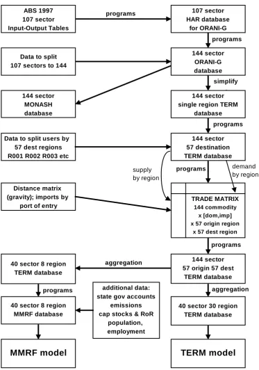
By contrast TERM offers a strategy, depicted in Figure 6, to estimate its database from very limited regional data. We describe below some key features of this strategy as applied to the Australian TERM model with base year of 19976.

(a) The process starts with a national input-output table and certain regional data. The minimum re-quirements for regional data are very modest: the distribution between regions of industry out-puts and of final demand aggregates. This distribution can be conceived as a set of regional shares, which may in turn be based on value data, or on physical units (eg, tonnes of wheat) or on numbers employed. This flexibility (regarding units) greatly increases the amount of data which may be used. Additional regional detail, such as region-specific technologies or con-sumption preferences may be added selectively, when available.

(b) The process is automated, so that additional detail can easily be added at a later stage.

(c) The database is constructed at the highest possible level of detail: 144 sectors and 57 regions. Aggregation (for computational tractability) takes place at the end of the process, not at the be-ginning. Perhaps surprisingly, the high level of disaggregation is often helpful in estimating missing data. When aggregated, the model database displays a richness of structure that belies the simple mechanical rules that were used to construct its disaggregated parent. For example, even though we normally assume that a given disaggregated sector has the same input-output coefficients wherever it is located, aggregated sectors display regional differences in technol-ogy. Thus, sectoral detail partly compensates for missing regional data7.

Our technique of combining a national IO table with limited regional data to produce a detailed in-ter-regional table bears many similarities to methods developed over several decades by regional IO modellers. Indeed, published regional input-output tables may well be in part constructed rather than observed. Unfortunately the method of construction may be poorly documented or unrepeat-able. The TERM data programs are downloadable and may easily be be customized to suit particu-lar needs. They will appeal to the modeller who would prefer to construct a multi-regional database using known assumptions, rather than rely on data constructed somehow by others.

Of course, published regional input-output tables may well form part of the inputs to the TERM data process. But they should certainly not constrain the degree of regional or sectoral detail that we aim for.

6

A more detailed description is given in Wittwer and Horridge (2010). However, that paper describes a later edition of the Australian TERM database, which distinguishes more sectors (172 rather than 144) and many more regions (206 rather than 57). The greater regional detail relies on census data that shows employment by sector and small region. The later edition also benefits from more detailed (four-digit) merchandise trade data for 60 ports.

7

(14)

5.3. The national input-out database

As shown in Figure 6, the TERM data process starts from the 1997 Australian input-output Tables, distinguishing 107 sectors. Our first step was to convert these tables to the file format of ORANI-G, a standard single-country CGE model. Next, working at the national level, we expanded the 107 sectors to 144. In choosing to split sectors, we hoped to avoid infelicities of classification that have caused problems in the past (such as the lumping together of exports of sugar, cotton and prawns) and also to split up sectors which showed regional differences in input mix or sales pattern. For ex-ample, we split up electricity generation according to the fuel used (which differs among Australian regions) and added considerable agricultural detail. The interests of one collabarator led to a re-markably detailed treatment of the wine and grape sectors, which were divided according to quality (some regions produce high-quality wine for export, others a cheaper brew for local drinking).

The main source for the sectoral split was unpublished ABS commodity cards data. Such data provide a split of sales for approximately 1,000 commodities to 107 industries, plus final users. However, the cards data do not always provide a desirable split from the 107 industries to the eventual 144 sectors of the disaggregated database. For example, there are significant sales of sug-arcane to the other food products sector (107-sector aggregation). We allocated all sugsug-arcane sales to refined sugar and zero sales to the seafood and other food products in our 144-sector disaggrega-tion. When the intermediate sales split was less obvious, we used activity weights of the purchasing sectors for the split.

The 144-sector national database has an independent value for our modelling work (for exam-ple, it forms the bulk of the MONASH database). For TERM purposes it was converted to a simpler format prior to the addition of regional detail.

5.4. Estimates of the regional distribution of output and final demands

The next step was to obtain, for each industry and final demander, an estimate of each statistical division’s share of national activity (these shares are the R001, R002, etc, of Figure 6). To develop a full input-output table for each region, we required estimates of industry shares (i.e., each region’s share of national activity for a given industry), industry investment shares, household expenditure shares, international export and import shares, and government consumption shares.

The main data sources for the industry split were:

• AgStats data from ABS, which details agricultural quantities and values at the SD level;

• employment data by industry at the SD level prepared by our colleague Tony Meagher from ABS census data and surveys;

• published ABS manufacturing census data (state level); and

• state yearbooks (for mining, ABS 1301, and for grapes and wine, ABS 1329.0).

Our sectoral split included a split of electricity into generation by fuel type plus a distribution sector. We relied on the internet sites of various electricity and energy agencies for capacity levels, on which shares of national activity were based.

Manufacturing, mining and services data disaggregated at the statistical division level were in quantities rather than values. These were adjusted these to fit state account sector aggregates (ABS 5220.0), as wages and industry composition vary between states. Industry investment shares are similar to industry activity shares for most sectors. Exceptions include residential construction input shares, set equal to ownership of dwellings investment shares in each statistical division.

Published ABS data (Tables 4 and 5, ABS 6530.0) provide sufficient commodity disaggrega-tion for the task of splitting regional consumpdisaggrega-tion aggregates into commodity shares. Such data also provide a split between capital city regions and other regions within each state.

(15)

exit with reasonable accuracy for that state. For other states, port activity is less complex, with most manufacturing trade passing through capital city ports and regional ports specialising in mineral and grain shipments.

State accounts data provide aggregated Commonwealth and state government spending in each region (ABS 5220.0). Employment numbers by statistical division for government administration and defence provide a useful split for these large public expenditure items. For other commodities, population shares by statistical division were used to calculate the distribution of Commonwealth and state government spending across regions.

By applying these shares to the national CGE database, we were able to compute the USE, FACTOR, and MAKE matrices on the left-hand side of Figure 1. None of these matrices distin-guish the source region of inputs.

5.4.1. Region-specific technology and output mix

By default, applying regional output shares to a national dataset leads to industry technologies that do not vary by region. That assumption would be very crude, were it not for the fact that very many sectors are distinguished during data construction. For example, it seems reasonable to assume that Bananas are grown in the same way in those (few) regions that they grow. It would be less reason-able to assume that "Agriculture" had the same technology.

Within Australia, some regions generate electricity with black coal (which is internationally traded), some with brown coal (which is too bulky to ship). The difference is important as brown coal emits far more CO2. To accommodate the regional technology difference, we distinguished separate brown-coal and black-coal electricity sectors—which each had uniform technology over regions. However, any one region used only one of the technologies. Prior to simulation we could aggregate together brown-coal and black-coal electricity sectors to produce a single electricity sec-tor which burns brown coal in some regions, black coal in others.

A related strategy is used to capture regional variation in crop mix. During the data-building process we usually distinguish a large number of crops, each of which is a single product industry. Thus we avoid complications by assuming a diagonal MAKE matrix. Prior to simulation we may aggregate together various agricultural industries, whilst leaving the associated commodities sepa-rate. The effect is that the input technology of "Agriculture" varies by region, as does the crop mix. Moreover, inputs such as land and labour can be switched between between crops, facilitating the analysis of land use change.

5.5. The TRADE matrix

The next stage was to construct the TRADE matrix on the right-hand side of Figure 1. For each commodity either domestic or imported, TRADE contains a 57x57 submatrix, where rows corre-spond to region of origin and columns correcorre-spond to region of use. Diagonal elements show pro-duction which is locally consumed. As shown in Figure 6 we already know both the row totals (supply by commodity and region) and the column totals (demand by commodity and region) of these submatrices. For Australia, hardly any detailed data on inter-regional state trade is available. We used the gravity formula (trade volumes follow an inverse power of distance) to construct trade matrices consistent with pre-determined row and column totals. In defence of this procedure, two points should be noted:

• Wherever production (or, more rarely, consumption) of a particular commodity is concentrated in one or a few regions, the gravity hypothesis is called upon to do very little work. Because our sectoral classification was so detailed, this situation occurred frequently.

• Outside of the state capitals, most Australian regions are rural, importing services and manu-factured goods from the capital cities, and exporting primary products through a nearby port. For a given rural region, one big city is nearly always much closer than any others, and the port of exit for primary products is also well defined. These facts of Australian geography again re-duce the weight borne by the gravity hypothesis.

(16)

V(r,d) = λ(r).μ(d).V(r,*).V(*,d) /D(r,d)2 r≠d where

V(r,d) = value of flow from r to d (corresponding to matrix TRADE in Fig. 1) V(r,*) = production in r (known)

V(*,d) = demand in d (known) D(r,d) = distance from r to d

The λ(r) and μ(d) are constants chosen to satisfy:

ΣrV(r,d)= V(*,d) and ΣdV(r,d)= V(r,*).

For TERM, the formula above gave rather implausible results, especially for service commodities. Instead we set:

V(r,d)/V(*,d) ∝ V(r,*)/D(r,d)k r≠d

where K is a commodity-specific parameter valued between 0.5 and 2, with higher values for com-modities not readily tradable. Diagonal cells of the trade matrices were set according to:

V(d,d)/V(d,*) = locally-supplied demand in d as share of local production = MIN{ V(d,*)/V(*,d),1} × F

where F is a commodity-specific parameter valued between 0.5 and 1, with a value close to 1 if the commodity is not readily tradable.

The initial estimates of V(r,d) were then scaled (using a RAS procedure) so that:

ΣrV(r,d)= V(*,d) and ΣdV(r,d)= V(r,*).

Transport costs as a share of trade flows were set to increase with distance: T(r,d)/V(r,d) ∝ D(r,d)

where T(r,d) corresponds to the matrix TRADMAR in Fig. 1. Again, the constant of proportionality is chosen to satisfy constraints derived from the initial national IO table.

(17)

Figure 4: Statistical divisions in Australia

5.6. Aggregation

Even though TERM is computationally efficient, it would be slow to solve if a full 144-sector, 57-region database were used. The next stage in the data procedure is to aggregate the data to a more manageable size. This stage is automated and effortless. The aggregation choice is application-specific. For example, to analyse the effects of drought we might choose a sectoral aggregation that retained detail in the agricultural and agriculture-related sectors, while grouping manufacturing and service industries broadly.

(18)

Figure 5: Aggregating from master database to policy simulation (watershed) regions

(19)

Figure 6: Producing regional databases for MMRF and TERM

TRADE MATRIX

144 commodity x [dom,imp] x 57 origin region

x 57 dest region

ABS 1997 107 sector Input-Output Tables

107 sector HAR database

for ORANI-G

Data to split 107 sectors to 144

144 sector ORANI-G database

144 sector MONASH database

40 sector 8 region MMRF database

144 sector single region TERM

database

40 sector 8 region TERM database

40 sector 30 region TERM database

144 sector 57 destination TERM database

144 sector 57 origin 57 dest

TERM database

TERM model MMRF model

Data to split users by 57 dest regions R001 R002 R003 etc

aggregation

aggregation programs

programs programs

simplify

programs

supply by region

programs

additional data: state gov accounts

emissions cap stocks & RoR

population, employment Distance matrix

(gravity); imports by port of entry

(20)

6. Conclusion: applications and developments of TERM

The TERM framework, developed originally for comparative static analyses of Australian issues, has been extended in several directions.

• It has been applied to several other countries, including Brazil, China, Finland, Indonesia, South Africa, Poland, USA and Japan. An Italian version is planned.

• Dynamic or multiperiod versions of TERM have been constructed for Australia, Brazil and Finland.

• The South African and Brazilian versions distinguish several household types, to focus on in-come distribution. One Brazilian version drives a large microsimulation database, distinguishing 100,000 households.

• Another Brazilian version focuses on land use, dividing land into four main types in each re-gion. The aim is to analyse whether increased export and biofuel demand for crops is compati-ble with preserving Amazon rainforests.

• TERM's capacity to model region-specific supply-side shocks in small regions has proved use-ful in modelling the effects of natural disasters such as earthquakes, droughts or crop diseases. The web page http://www.monash.edu.au/policy/term.htm links to a number of these versions.

(21)

References

ABS 2002 (and previous issues), Australian National Accounts: State Accounts, Catalogue 5220.0, Canberra.

Adams, P., Horridge, M. and Wittwer, G. 2002, MMRF-Green: A dynamic multi-regional applied general equilibrium model of the Australian economy, based on the MMR and MONASH models, Prepared for the Regional GE Modelling Course, 25-29 November 2002.

Dixon, P., B. Parmenter and D. Vincent 1978, "Regional Developments in the ORANI Model", in R. Sharpe (ed. ), Papers of the Meeting of the Australian and New Zealand Section Regional Sci-ence Association, Third Meeting, Monash University, pp. 179-188.

Dixon, P., Parmenter, B.,Sutton, J. and Vincent, D. 1982, ORANI: A Multisectoral Model of the Australian Economy, North-Holland, Amsterdam.

Flegg, A. & Tohmo, T. (2008), Regional input-output models and the FLQ formula: a case study of Finland, Discussion Paper 0808, Department of Economics, University of the West of England. Flegg, A., Webber, C. & Elliott, M. (1995), On the appropriate use of location quotients in

gener-ating regional input-output tables, Regional Studies, 29, 547-561.

Giesecke, J. 1997, The FEDERAL-F model, CREA Paper No. TS-07, Centre for Regional Eco-nomic Analysis, University of Tasmania, November.

Higgs, P., B. Parmenter and R. Rimmer 1988, "A Hybrid Top-Down, Bottom-Up Regional Com-putable General Equilibrium Model", International Science Review, Vol. 11, No. 3, 1988, pp. 317-328.

Horridge, J.M., Madden, J.R. and G. Wittwer (2005), "The impact of the 2002-03 drought on Aus-tralia", Journal of Policy Modeling, Vol 27/3, pp. 285-308.

Liew, L. 1984, "Tops-Down" Versus "Bottoms-Up" Approaches to Regional Modeling, Journal of Policy Modeling, Vol. 6, No. 3, pp. 351-368.

Madden, J. 1990, FEDERAL: a two-region multi-sectoral fiscal model of the Australian economy, Ph.D. thesis, University of Tasmania, Hobart.

Maddock, R. and McLean, I. 1987, “The Australian economy in the very long run”, chapter 1 in Maddock, R. and McLean, I. (editors), The Australian Economy in the Long Run, Cambridge University Press.

Naqvi, F. and Peter, M. 1996, “A Multiregional, Multisectoral model of the Australian Economy with an Illustrative Application”, Australian Economic Papers, 35:94-113.

Pearson, K. 1988, “Automating the Computation of Solutions of large Economic Models”, Eco-nomic Modelling, 7:385-395.

Peter, M., Horridge, M. Meagher, G.A., Naqvi, F. and Parmenter, B.R.,1996, The Theoretical Structure of MONASH-MRF, CoPS/Impact Working Paper OP-85,June 1996

from: http://www.monash.edu.au/policy/elecpapr/op-85.htm