Tight Security of Cascaded
LRW2
Ashwin Jha and Mridul Nandi
Indian Statistical Institute, Kolkata, India
{ashwin.jha1991,mridul.nandi}@gmail.com
Abstract. At CRYPTO ’12, Landecker et al. introduced the cascaded LRW2(orCLRW2) construction, and proved that it is a secure tweakable block cipher up to roughly 22n/3queries. Recently, Mennink presented a distinguishing attack onCLRW2in 2n1/223n/4queries. In the same paper, he discussed some non-trivial bottlenecks in proving tight security bound, i.e. security up to 23n/4 queries. Subsequently, he proved security up to 23n/4 queries for a variant of CLRW2 using 4-wise independent AXU assumption and the restriction that each tweak value occurs at most 2n/4times. Moreover, his proof relies on a version of mirror theory which is yet to be publicly verified. In this paper, we resolve the bottlenecks in Mennink’s approach and prove that the originalCLRW2 is indeed a secure tweakable block cipher up to roughly 23n/4queries. To do so, we develop two new tools: First, we give a probabilistic result that provides improved bound on the joint probability of some special collision events; Second, we present a variant of Patarin’s mirror theory in tweakable permutation settings with a self-contained and concrete proof. Both these results are of generic nature, and can be of independent interests. To demonstrate the applicability of these tools, we also prove tight security up to roughly 23n/4queries for a variant ofDbHtS, calledDbHtS-p, that uses two independent universal hash functions.
Keywords: LRW2,CLRW2, tweakable block cipher, mirror theory
1
Introduction
Tweakable Block Ciphers: A tweakable block cipher (or TBC for short) is a
cryptographic primitive that has an additional public indexing parameter called tweak in addition to the usual secret key of a standard block cipher. This means that a tweakable block cipher,Ee:K × T × M → M, is a family of permutations
on the plaintext/ciphertext spaceMindexed by two parameters: the secret key k ∈ K and the public tweakt ∈ T. Liskov, Rivest, and Wagner formalized the concept of TBCs in their renowned work [1]. Tweakable block ciphers are more versatile than a standard block cipher and find a broad range of applications, most notably in authenticated encryption schemes, such as TAE [1], ΘCB [2] (TBC-based generalization of the OCBfamily [3,2,4]), PIV[5], COPA [6], SCT
[7] (used inDeoxys [8,7]),AEZ [9] etc.; and message authentication codes, such
asPMAC TBC3KandPMAC TBC1K[10],PMAC2xandPMACx[11],ZMAC[12],
Birthday-Bound Secure TBCs: Although there are some TBC
construc-tions designed from scratch, notably Deoxys-BC [8] and Skinny [8,22], still the wide availability of secure and well-analyzed block ciphers make them perfect candidates for constructing TBCs. In [1], Liskov et al. proposed two construc-tions for TBCs based on a secure block cipher. The second construction, called
LRW2, is defined as follows:
LRW2((k, h), t, m) =E(k, m⊕h(t))⊕h(t),
whereE is a block cipher,kis the block cipher key, andhis an XOR universal hash function. TheLRW2 construction is strongly related to theXEX construc-tion by Rogaway [2], and its extensions by Chakraborty and Sarkar [23], Mine-matsu [24], and Granger et al. [25]. All these schemes are inherently birthday bound secure due to the internal hash XOR collisions, i.e. the adversary can choose approx. 2n/2 queries in such a way that there will be two queries (t, m) and (t0, m0) withm⊕h(t) = m0⊕h(t0). This leads to a simple distinguishing event c⊕c0=m⊕m0.
Beyond-the-Birthday Bound Secure TBCs: In [26], Landecker et al. first
suggested the cascading of two independent LRW2 instances to get a beyond-the-birthday bound (BBB) secure TBC, called CLRW2, i.e.
CLRW2((k1, k2, h1, h2), t, m) =LRW2((k2, h2), t,LRW2((k1, h1), t, m)).
They proved thatCLRW2is a secure TBC up to approx. 22n/3 queries. Later on Procter [27] pointed out a flaw in the security proof of CLRW2. The proof was subsequently fixed by both Landecker et al. and Procter to recover the claimed security bounds. Lampe and Seurin [28] studied the`≥2 independent cascades of LRW2, and proved that it is secure up to approx. 2``n+2 queries. They further conjectured that the `cascade is secure up to 2``n+1 queries. Recently, Mennink [29] showed a 2n1/223n/4-query attack on CLRW2. In the same paper he also proved security up to 23n/4 queries, albeit for a variant of CLRW2 with strong assumptions on the hash functions and restrictions on tweak repetitions.
All of the above constructions are proved to be secure in standard model. However, there are TBC constructions in public random permutation and ideal cipher model as well. In [13], Cogliati, Lampe and Seurin introduced the tweak-able Even-Mansour construction and its cascaded variant. They showed that the two round construction is secure up to approx. 22n/3queries. A simple corollary of this result also gives security ofCLRW2up to 22n/3queries. The bound is tight in the ideal permutation model as one can simply fix the tweak and use the 22n/3 queries attack on key alternating cipher by Bogdanov et al. [30]. Some notable BBB secure TBC constructions in the ideal cipher model include, Mennink’s
˜
F[1] and˜F[2] [31,32], Wang et al. 32 constructions [33], and their generalization, called XHX, by Jha et al. [34]. All of these constructions are at most birthday bound secure in the sum of key size and block size.1 Recently, Lee and Lee [35] proved that a two level cascade of XHX, calledXHX2, achieves BBB security in terms of the sum of key size and block size.
1 ˜
1.1 Recent Developments in the Analysis of CLRW2
In [29], Mennink presented an improved security analysis of CLRW2. The major contribution was an attack in approx. n1/223n/4 queries. The attack works by finding 4 queries (t, m1, c1), (t0, m2, c2), (t, m3, c3), and (t0, m4, c4) such that
AltColl
(
h1(t)⊕m1=h1(t0)⊕m2 ∧ h2(t0)⊕c2=h2(t)⊕c3 h1(t)⊕m3=h1(t0)⊕m4 ∧ h2(t0)⊕c4=h2(t)⊕c1.
This leads to a simple distinguishing attack since, in case of CLRW2,
m1⊕m2⊕m3⊕m4= 0 =c1⊕c2⊕c3⊕c4,
happens with probability 1, givenAltCollholds. In contrast this happens with probability close to 1/2n for an ideal tweakable random permutation.
Following on the insights from the attack, Mennink [29] also gives a security proof of the same order for a variant of CLRW2. Basically, the proof bounds the probability that the above given four equations hold. Additionally, inspired by [36], Patarin’s mirror theory [37,38,39] is used which requires a bound on the probability of some more bad events. The major bottleneck in proving the security beyond 22n/3queries comes from two directions:
– First, there is no straightforward way of proving the upper bound of the prob-ability of occurrence ofAltColl to 2q34n, where q is the number of queries. This is due to two reasons: (1) the adversary has full control over the tweak usages; and (2) the hash functions are just 2-wise independent XOR univer-sal.
– Second, mirror theory was primarily developed to lower bound the number of solutions to equations arising for some random system which is trying to mimic a random function. This is not the case here, and as we will see in later sections, the mirror theory bound is directly dependent on tweak repetitions.
In order to bypass the two bottlenecks, following assumptions are made in [29]: 1. The hash functions are 4-wise independent AXU.
2. The maximum number of tweak repetitions is restricted to 2n/4. 3. A limited variant of mirror theory result is true for q <23n/4.
Among the three assumptions, the first two are at least plausible. But the last assumption is questionable as barring certain restricted cases, the proof of mirror theory has many gaps which are still open or unproven, as has been noted in [40,41].
1.2 Contributions of this Work
1. The Alternating Events Lemma: We derive a generic tool (see section4) to bound the probability of events of the formAltColl. InCLRW2analysis only a special case is required, where the randomness comes from two independent universal hash functions.
2. Mirror Theory in Tweakable Permutation Setting:We adapt the mirror the-ory line of argument (see section 5) to get suitable bounds in tweakable permutation setting. This is a generalization of the existing mirror theory result in function setting.
Using the above mentioned tools we prove thatCLRW2is secure up to approx. 23n/4 queries (see section6). Our result, in combination with the attack in [29] (see supplementary material B), gives the tight (up to a logarithmic factor) security of CLRW2.
As a side-result on the application of our tools, we also prove tight security up to roughly 23n/4 queries for a variant of DbHtS [42], called DbHtS-p, that uses two independent universal hash functions (see section7).
Here, we explicitly remark that our bound onCLRW2is not derivable from the recent result onXHX2[35].
2
Preliminaries
Notational Setup: Forn∈ N, [n] denotes the set {1,2, . . . , n}, {0,1}n
de-notes the set of bit strings of length n, andPerm(n) denotes the set of all per-mutations over{0,1}n. Forn, κ∈
N,BPerm(κ, n) denotes the set of all families
of permutationsπk :=π(k,·)∈Perm(n), indexed byk∈ {0,1}κ. We sometimes
extend this notation, whereby BPerm(κ, τ, n) denotes the set of all families of permutationsπ(k,t), indexed by (k, t)∈ {0,1}κ× {0,1}τ. Forn, r∈N, such that n≥r, we define the falling factorial (n)r:=n!/(n−r)! =n(n−1)· · ·(n−r+ 1).
For q ∈ N, xq denotes the q-tuple (x
1, x2, . . . , xq), and xb
q denotes the set
{xi : i ∈ [q]}. By an abuse of notation we also use xq to denote the multiset
{xi:i∈[q]}andµ(xq, x0) to denote the multiplicity ofx0 ∈xq. For a setI ⊆[q]
and a q-tuple xq, xI denotes the tuple (x
i)i∈I. For a pair of tuples xq and yq, (xq, yq) denotes the 2-ary q-tuple ((x1, y1), . . . ,(x
q, yq)). An n-ary q-tuple
is defined analogously. For q ∈ N, for any set X, (X)q denotes the set of all
q-tuples with distinct elements fromX. Forq∈N, a 2-ary tuple (xq, yq) is called
permutation compatible, denotedxq
!yq, ifx
i=xj ⇐⇒ yi=yj. Extending
notations, a 3-ary tuple (tq, xq, yq) is called tweakable permutation compatible, denoted by (tq, xq)!(tq, yq), if (ti, xi) = (tj, xj) ⇐⇒ (ti, yi) = (tj, yj). For
any tuple xq ∈ Xq, and for any functionf : X → Y, f(xq) denotes the tuple
(f(x1), . . . , f(xq)). We use short hand notation∃∗to represent the phrase “there
exists distinct”.
2.1 Some Useful Inequalities
Definition 2.1. Forr≥s, let a= (ai)i∈[r] andb = (bj)j∈[s] be two sequences over N. We say that acompresses tob, if there exists a partition P of [r] such that P contains exactlyscells, say P1, . . . ,Ps, and∀i∈[s], bi=Pj∈Piaj. Proposition 1. Forr≥s, leta= (ai)i∈[r] andb= (bj)j∈[s] be sequences over
N, such thata compresses to b. Then for any n∈ N, such that 2n ≥Pri=1ai,
we have Qri=1(2n)ai≥
Qs j=1(2
n) bj.
In [34, Proof of Lemma 3], the authors refer to a variant of Proposition1. We remark that, this variant [34, Fact 1] is in fact false. However, [34, Proof of Lemma 3] implicitly used Proposition1, and hence stands correct.
Proposition 2. Forr ≥2, let c = (ci)i∈[r] andd= (di)i∈[r] be two sequences overN. Let a1, a2, b1, b2 ∈N, such thatci≤aj,ci+di ≤aj+bj for all i∈[r]
andj∈[2], andPri=1di=b1+b2. Then, for anyn∈N, such thataj+bj ≤2n
forj∈[2], we have Qri=1(2n−c
i)di ≥(2
n−a1)
b1(2
n−a2)
b2.
Proposition 2 is quite intuitive, in the sense, that the starting value in each of the falling factorial term on the left is at least as much as the starting values on the right, and the total number of terms are same on both the sides. The formal proofs of Proposition 1and2 are given in supplementary materialA.
2.2 (Tweakable) Block Ciphers and Random Permutations
A block cipher with key size κ and block size n is a family of permutations E ∈ BPerm(κ, n). For k ∈ {0,1}κ, we denoteE
k(·) :=E(k,·), and Ek−1(·) :=
E−1(k,·). A tweakable block cipher with key sizeκ, tweak sizeτand block sizen is a family of permutationsEe∈BPerm(κ, τ, n). Fork∈ {0,1}κ andt∈ {0,1}τ,
we denote Eek(t,·) := E(k, t,e ·), and Eek−1(t,·) := Ee−1(k, t,·). Throughout this
paper, we fixκ, τ, n∈Nas the key size, tweak size and block size, respectively,
of the given (tweakable) block cipher.
We say thatΠis an (ideal) random permutation on block space {0,1}n to
indicate that Π←$Perm(n). Similarly, we say that Πe is an (ideal) tweakable
random permutation on tweak space{0,1}τ and block space{0,1}n to indicate
that Πe←$BPerm(τ, n).
2.3 (T)SPRP Security Definitions
simulator. Let A(q, t) be the class of all non-trivial distinguishers limited to q oracle queries, andtcomputations.
(Tweakable) Strong Pseudorandom Permutation (SPRP): The SPRP advantage of distinguisher A againstE instantiated with a key K←${0,1}κ is
defined as
AdvsprpE (A) =AdvE±;Π±(A) :=
Pr
h
AEK±= 1i−PrhAΠ±= 1i
. (1)
The SPRP security of E is defined as AdvsprpE (q, t) := max
A∈A(q,t)Adv sprp
E (A).
Similarly, the TSPRP advantage of distinguisherA againstEe instantiated with
a key K←${0,1}κis defined as
Advtsprp e
E (A) =AdvEe±;eΠ±(A) :=
Pr
h
AEeK±= 1i
−PrhAeΠ±= 1i
. (2)
The TSPRP security ofEe is defined asAdv
tsprp
e
E (q, t) :=Amax∈A(q,t)Adv tsprp
e
E (A).
2.4 The Expectation Method
Let A be a computationally unbounded and deterministic distinguisher that tries to distinguish between two oracles O0 and O1 via black box interaction with one of them. We denote the query-response tuple of A’s interaction with its oracle by a transcript ω. This may also include any additional information the oracle chooses to reveal to the distinguisher at the end of the query-response phase of the game. We denote by Θ1 (res. Θ0) the random transcript variable when A interacts with O1 (res.O0). The probability of realizing a given tran-script ω in the security game with an oracle O is known as the interpolation probability of ω with respect to O. Since A is deterministic, this probability depends only on the oracleOand the transcriptω. A transcriptω is said to be attainable if Pr [Θ0=ω]> 0. The expectation method (stated below) is quite useful in obtaining improved bounds in many cases [43,44,45]. The H-coefficient technique due to Patarin [46] is a simple corollary of this result where the ratio is a constant function.
Lemma 2.1 (Expectation Method [43]).LetΩbe the set of all transcripts. For somebad>0and a non-negative functionratio:Ω→[0,∞), suppose there is a setΩbad⊆Ω satisfying the following:
– Pr [Θ0∈Ωbad]≤bad;
– For anyω /∈Ωbad,ω is attainable and
Pr [Θ1=ω] Pr [Θ0=ω]
≥1−ratio(ω).
Then for an distinguisher A trying to distinguish between O1 andO0, we have the following bound on its distinguishing advantage:
2.5 Patarin’s Mirror Theory
In [37] Patarin defines Mirror theory as a technique to estimate the number of solutions of linear systems of equalities and linear non equalities in finite groups. In its most general case, the mirror theory proof is tractable up to the order of 22n/3 security bound, but it readily becomes complex and extremely difficult to verify, as one aims for the optimal bound [40,41]. We remark here that this in no way suggests that the result is incorrect, and in future, we might even get some independent verifications of the result.
We restrict ourselves to the binary field Fn
2 with ⊕ as the group opera-tion. We will use the Mennink and Neves interpretation [36] of mirror theory. For ease of understanding and notational coherency, we sometimes use different parametrization and naming conventions. Let q≥1 and let L be the system of linear equations
{e1:Y1⊕V1=λ1, e2:Y2⊕V2=λ2, . . . , eq :Yq⊕Vq =λq}
where Yq and Vq are unknowns, and λq ∈ ({0,1}n)q are knowns. In addition
there are (in)equality restrictions onYq and Vq, which uniquely determine b
Yq
and Vbq. We assume that Ybq and Vbq, are indexed in an arbitrary order by the
index sets [qY] and [qV], where qY = |Ybq| and qV = |Vbq|. This assumption
is without any loss of generality as this does not affect the system L. Given such an ordering, we can view Ybq and Vbq as ordered sets {Y10, . . . , Yq0Y} and {V0
1, . . . , Vq0V}, respectively. We define two surjective index mappings:
ϕY : (
[q]→[qY]
i7→j if and only ifYi=Yj0.
ϕV : (
[q]→[qV]
i7→kif and only ifVi=Vk0.
It is easy to verify that L is uniquely determined by (ϕY, ϕV, λq), and
vice-versa. Consider a labeled bipartite graph G(L) = ([qY],[qV],E) associated with
L, where E ={(ϕY(i), ϕV(i), λi) :i ∈[q]}, λi being the label of edge. Clearly,
each equation inLcorresponds to a unique labeled edge (assuming no duplicate equations). We give three definitions with respect to the systemLusingG(L).
Definition 2.2 (cycle-freeness).Lis said to be cycle-free if and only ifG(L) is acyclic.
Definition 2.3 (ξmax-component).Two distinct equations (or unknowns) in L are said to be in the same component if and only if the corresponding edges (res. vertices) inG(L)are in the same component. The size of any componentC inL, denotedξ(C), is the number of vertices in the corresponding component of G(L), and the maximum component size is denoted byξmax(L)(or simplyξmax).
Theorem 2.1 (Fundamental Theorem of Mirror Theory [37]). LetL be a system of equations over the unknowns(Ybq,Vbq), that is (i) cycle-free, (ii)
non-degenerate, and (iii)ξ2
max·max{qY, qV} ≤2n/67. Then, the number of solutions
(y1, . . . , yqY, v1, . . . , vqV)of L, denoted hq, such that yi6=yj andvi 6=vj for all i6=j, satisfies
hq ≥
(2n)qY(2
n) qV
2nq . (3)
A proof of this theorem is given in [37]. As mentioned before, the proof is quite involved with some claims remaining open or unproved. On the other hand, the same paper contains results for various other cases. For instance, for ξ = 2, several sub-optimal bounds have been shown. By sub-optimal, we mean that a factor of (1−), for some >0, is multiplied to the right hand side of Eq. (3). Inspired by this, we give the following terminology which will be useful in later references to mirror theory.
For ξ ≥ 2, > 0, we write (ξ, )-restricted mirror theory theorem to denote the mirror theory result in which the number of solutions,hq, of
a system of equations withξmax=ξ, satisfieshq ≥(1−)
(2n)qY(2n)qV 2nq . Mirror theory has been primarily used for bounding the pseudorandomness of sum of permutations [47,48,37,40] with respect to a random function. For in-stance, suppose we sample elements inYbq andVbqas outputs of two independent
random permutations Π1 and Π2, respectively, over qY and qV distinct inputs,
respectively. Let pr1 be the probability of realizing the system of equations L, and pr0 be the probability of realizing the q-tuple λq through random function
outputs overqdistinct inputs. Then, it is easy to see thatpr1=hq/(2n)qY(2
n) qV and pr0 = 1/2nq. Clearly, the above given lower bound on h
q implies that pr1 ≥ (1−)pr0. When combined with the H-coefficient technique, we get an term in the distinguishing advantage bound for sum of random permutations. Herecan be viewed as the degree of deviation from random function behavior. This is precisely the reason that one finds terms of the form (2n)qY(2
n)
qV and
2nqin mirror theory bounds. We refer the readers to [37,36] for a more detailed exposition on the aim and motivations behind mirror theory.
In [29], (4,3q/2n)-restricted mirror theory theorem is used. In section5, we
study the (ξ, q4/23n) case, forξ≤2n/2qand present a variant of mirror theory
suitable for tweakable permutation scenario.
3
Revisiting Mennink’s Improved Bound on
CLRW2
We first describe the notion of`-wise independent XOR universal hash functions as given in [29]. This notion will be used for the description ofCLRW2(for`= 2), as well as Mennink’s improved bound on CLRW2(for`= 4).
Definition 3.1. For ` ≥2, ≥ 0, a family of functions H = {h : {0,1}τ →
, denoted -AXU`, if for anyj ∈ {2, . . . , `}, any tj ∈ ({0,1}τ)j and a δj−1 ∈
({0,1}n)j−1, we have
Pr [H←$H : H(t1)⊕H(t2) =δ1, . . . ,H(t1)⊕H(tj) =δj−1]≤j−1. (4) For`= 2, this is nothing but the notion of AXU hash functions, first introduced by Krawczyk [49] and later by Rogaway [50]. In [29], the author suggested a simple AXU`hash function family using finite field arithmetic for small domain
(τ=n). Basically, the hash function family is defined as follows
h(x) :=
`−1
M
i=1 hixi
forh= (h1, . . . , h`−1), wheredenotes field multiplication operator with respect to some irreducible polynomial over the binary fieldFn
2. For`= 2, this yields the popular polyhash function. In general, this function requires`−1 keys and`−1 field multiplications to achieve 2−n-AXU
`. Alternatively, secure block ciphers
can also be used to construct (2n−`+1)−1-AXU
`hash functions over sufficiently
large domains.
3.1 Description of the Cascaded LRW2 Construction
Let E ∈BPerm(κ, n) be a block cipher. LetHbe a hash function family from {0,1}τ to{0,1}n. We define the tweakable block cipher LRW2[E,H], based on
the block cipher E and the hash function familyH, by the following mapping: ∀(k, h, t, m)∈ {0,1}κ× H × {0,1}τ× {0,1}n,
LRW2[E,H](k, h, t, m) :=Ek(m⊕h(t))⊕h(t). (5)
For`∈N, the`-round cascadedLRW2construction, denotedCLRW2[E,H, `], is
a cascade of` independentLRW2 instances, i.e.CLRW2[E,H, `] is a tweakable block cipher, based on the block cipherEand the hash function familyH, defined as follows:∀(k`, h`, t, m)∈ {0,1}κ`× H`× {0,1}τ× {0,1}n,
yi:= (
LRW2[E,H](ki, hi, t, m) fori= 1, LRW2[E,H](ki, hi, t, yi−1) otherwise.
CLRW2[E,H, `](k`, h`, t, m) :=y
`. (6)
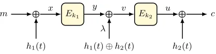
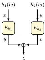
The 2-roundCLRW2, was first analyzed by Landecker et al. [26], whereas the` > 2 case was studied by Lampe and Seurin [28]. Since we mainly focus on the`= 2 case, we use the nomenclatures, CLRW2 and cascaded LRW2, interchangeably with 2-round CLRW2. Figure 3.1 gives a pictorial description of the cascaded
LRW2 construction. Throughout the rest of the paper, we use the notations from Figure 3.1in context ofCLRW2.
Ek1 ⊕
⊕⊕
m
h1(t)
⊕ ⊕⊕
h1(t)⊕h2(t)
Ek2 ⊕⊕⊕
h2(t)
c
x y
λ
v u
Fig. 3.1:The cascaded LRW2construction.
3.2 Mennink’s Proof Approach
The proof in [29] applies H-coefficient technique coupled with mirror theory. The main focus is to identify a suitable class of bad events on (xq, uq), whereqis the number of queries, which makes mirror theory inapplicable. Crudely, the bad events correspond to cases where for some query there is no randomness left (in the sampling of yq andvq) in the ideal world. Given a good transcript, mirror theory is applied to bound the number of solutions of the system of equation {Yi⊕Vi =λi:i∈[q]}, where Yi and Vi are unknowns satisfying xq !Yq and
Vq
!uq, andλq is fixed. The proof relies on three major assumptions: Assumption 1.His AXU4 hash function family.
Assumption 2. For anyt0 ∈ {0,1}τ,µ
t0 =µ(tq, t0)≤γ= 2n/4.
Assumption 3. 4,23qn
-restricted mirror theory theorem is correct.
Transcript Graph: A graphical view onxq anduq was used to characterize
all bad events. Basically, each transcript is mapped to a unique bipartite graph onxq, uq, as defined in Definition3.2.
Definition 3.2 (Transcript Graph). A transcript graphG= (X,U,E) asso-ciated with(xq, uq), denotedG(xq, uq), is defined asX :={(x
i,0) :i∈[q]}; U :=
{(ui,1) :i ∈ [q]}; andE := {((xi,0),(ui,1)) : i ∈ [q]}. We also associate the
value λi =h1(ti)⊕h2(ti) with edge((xi,0),(ui,1))∈ E.
Note that the graph may not be simple, i.e. it can contain parallel edges. For all practical purposes we may drop the 0 and 1 for (x,0)∈ X and (u,1)∈ U, as they can be easily distinguished from the context and notations. Further, for some i, j∈[q], ifxi=xj (orui=uj) , then they share the same vertexxi=xj=xi,j
(orui=uj=ui,j). The eventxi=xj andui=uj, although extremely unlikely,
will lead to a parallel edge in G. Finally each edge (xi, ui)∈ E corresponds to a
query indexi ∈[q], so we can equivalently view (and call) the edge (xi, ui) as
indexi. Figure3.2gives an example graph forG.
Bad Transcripts: A transcript graphG(xq, uq) is called bad if:
1. it has a cycle of size = 2.
2. it has two adjacent edgesiandj such thatλi⊕λj= 0.
3. it has a component with number of edges≥4.
x1
u1 u2
x2,3
u3
x4
u4
x5
u5,6
x6,7
u7,8
x8
u9 u10
x9,...,i
ui,i+1
xi+1
. . . . . . . . .
xi+2 xi+3
ui+2,...,q−4
xq−4
. . .. . .. . .
xq−3,q−2
uq−2,q−1
xq−1,q
uq−3,q
Fig. 3.2:A possible transcript graphG(xq, uq) associated with (xq, uq). Vertices inxq
are colored blue and vertices inuq are colored red, for illustration only.
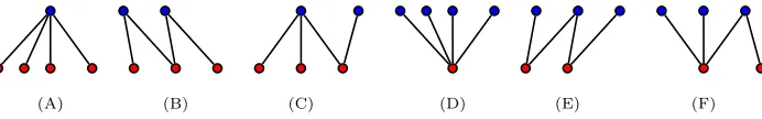
in the real world. Condition 3 may lead to a cycle of length ≥ 4 edges. The non-fulfillment of condition 1,2 and 3 satisfies the cycle-free and non-degeneracy properties required in mirror theory. It also boundsξmax≤4. Condition 1 and 2 contribute small and insignificant terms and can be ignored from this discussion. We focus on the major bottleneck, i.e. condition 3. The subgraphs corresponding to condition 3 are given in Figure 3.3. Configuration (D), (E), and (F) are symmetric to (A), (B), and (C). So we can study (A), (B), and (C), and the other three can be similarly analyzed.
(A) (B) (C) (D) (E) (F)
Fig. 3.3: Possible configuration of size = 4 edge subgraphs. Vertices inxq are colored blue and vertices inuq are colored red, and vertex labels are omitted for brevity.
Bottleneck 1: Bound on the probability of (A), (C), (D) and (F) —
This can be divided into two parts: (a) Configuration (A) arises for the event
∃∗i, j, k, lsuch thatxi=xj =xk=x`.
This event is upper bounded toq43 using assumption 1 on hash functions. Similar argument holds for (D).
(b) Configuration (C) (similarly for F) arises for the event
∃∗i, j, k, `∈[q] such that xi=xj=xk∧uk=u`.
In this case we can apply assumption 1 (even AXU3would suffice) to get an upper bound ofq43.
Bottleneck 2: Bound on the probability of (B) — Configuration (B)
arises for the event
∃∗i, j, k, lsuch that xi=xj∧uj=uk∧xk =x`.
precisely the case exploited in Mennink’s attack onCLRW2[29] (see supplemen-tary material B). In this case for a fixedi, j, k, `the probability is bounded by 2. There are at most q2 choices for (i, j), at most (µ
ti −1) choices for k and a single choice for`given i,j andk. Thus the probability is bounded byq2γ2 (using assumption 2). Similar argument holds for (E).
Bottleneck 3: Mirror theory bound — The final hurdle is the use of
mirror theory in computation of real world interpolation probability, which re-quires assumption 3. Yet another issue is the nature of the mirror theory bound. A straightforward application of mirror theory bound leads to a term of the form
Q t0∈
b tq(2n)µt0
2nq (1−O(q/2 n)),
in the ratio of interpolation probabilities (as required for H-coefficient technique), where P
t0∈
b
tqµt0 =q. The boxed expression (particularly, the numerator in the expression) is of main interest. In the worst case,µt0 =O(q), which gives a lower bound of the form 1−q2/2n for the boxed expression. But using assumption 2, we get a lower bound of 1−qγ/2n as µ
t0 ≤γ.
Severity of the assumptions in [29]. Among the three assumptions, assump-tion 1 and 2 are plausible in the sense that real life use-cases exist for assumpassump-tion 2 and practical instantiations are possible for assumption 1. Another point of note is the fact thatγ <2n/4is imposed due to bottleneck 3. Otherwise a better bound of γ <2n/2 could have been used. While assumption 1 and 2 are plau-sible to a large extent, assumption 3 is disputable. This is because no publicly verifiable proof exists for the generalized mirror theory. In fact, the proof for a special case of mirror theory also has some unproved gaps and mistakes. See Remark1 for one such issue.
Although the proof in [29] requires the above mentioned assumptions, the proof approach seems quite simple and in some cases it highlights the bottle-necks in getting tight security. In the remainder of this paper, we aim to resolve all the bottlenecks discussed here, while relaxing all the assumptions made in [29]. Specifically, bottleneck 2 is resolved using the tools from section 4, and bottlenecks 1 and 3 are resolved using the tools from sections 4 and 5, and a careful application of the expectation method in section6.
4
Results on (Multi)Collisions in Universal Hash
LetH={h| h:T → B}be a family of functions. A pair of distinct elements (t, t0) from T is said to be colliding for a function h ∈ H, if h(t) = h(t0). A family of functions H={h| h:T → B} is called an -universal hash if for all t6=t0∈ T,
Throughout this section, we fixtq = (t
1, . . . , tq)∈(T)q. For a randomly chosen
hash function H←$H, the probability of having at least one colliding pair intq
is at most q2
·. This is straightforward from the union bound.
4.1 The Alternating Collisions and Events Lemmata
SupposeHis an-universal hash andH1,H2←$Hare two independently drawn universal hash functions. Then, by applying independence and union bound, we have
Pr [∃∗i, j, k∈[q], H1(ti) =H1(tj) ∧ H2(tj) =H2(tk)]≤q(q−1)(q−2)·2.
Now we go one step further. We would like to bound the probability of the following event:
∃∗i, j, k, l∈[q], H
1(ti) =H1(tj) ∧ H2(tj) =H2(tk) ∧ H1(tk) =H1(tl).
For any fixed distinct i, j, k andl, we cannot claim that the probability of the event H1(ti) =H1(tj) ∧ H2(tj) =H2(tk) ∧ H1(tk) =H1(tl) is3 as the first
and last event are no longer independent. Now, we show how we can get an improved bound even in the dependent situation. In particular, we prove the following lemma.
Lemma 4.1 (Alternating Collisions Lemma).SupposeH1,H2←$Hare two independently drawn universal hash functions andtq∈(T)
q. Then,
Pr [∃∗i, j, k, l∈[q],H1(ti) =H1(tj)∧ H1(tk) =H1(tl)∧ H2(tj) =H2(tk)]≤q21.5.
Proof. For anyh∈ H, we define the following useful set:
Ih={(i, j) :h(ti) =h(tj)}.
Let us denote the size of the above set byIh. So, Ih is the number of colliding
pairs for the hash functions h. We also define a set H≤ = {h : Ih ≤ √1}
which collects all hash functions having a small number of colliding pairs. We denote the complement set by H>. Now, by using double counting of the set
{(h, i, j) :h(ti) =h(tj)} we get
X
h
Ih≤q(q−1)·· |H|. (8)
Basically for every h, we have exactly Ih choices of (i, j) and so the size of
the set {(h, i, j) : h(ti) = h(tj)} is exactly PhIh. On the other hand, for any
1 ≤ i < j ≤ q, there are at most · |H| hash functions h, such that (ti, tj)
is a colliding pair for h. This follows from the definition of the universal hash function. From Eq. (8) and the definition ofH≤, we have
|H>|
√ +
X
h∈H≤ Ih ≤
X
h
Let E denote the event that there exists distinct i, j, k, l such that H1(ti) = H1(tj) ∧ H1(tk) =H1(tl) ∧ H2(tj) =H2(tk). Now, we proceed to bound the
probability of this event.
Pr [E] =X
h
Pr [E∧H1=h]
=X
h
Pr [H1=h]×Pr [E∧H1=h|H1=h]
1
≤X
h
Pr [H1=h]×min{1, Ih2·}
= Pr [H1∈ H>] + X
h∈H≤
Pr [H1=h]·Ih2·
2 ≤ |H>|
|H| +
X
h∈H≤ Ih·
√ |H| .
= √
|H|×
|H>|
√ +
X
h∈H≤ Ih
3
≤q(q−1)1.5.
First, we justify inequality 1. Given H1 = h, the probability of the event E is same as the probability of the following event:
∃∗(i, j),(k, l)∈ I
h,H2(tj) =H2(tk).
There are at mostI2
h pairs of pairs and for each pair of pairs and the collision
probability of H2(tj) = H2(tk) is at most . So probability of the above event
can be at most min{1, I2
h ·}. Now, we justify inequality 2 using two facts.
First,H1←$H, i.e. Pr [H1=h] =|H|−1 for all h∈ H. Second, for all h∈ H≤, Ih≤1/
√
. Inequality 3 follows from Eq. (9). ut
Now, we generalize the above result for a more general setting. The proof of the result is similar to the previous proof and hence we skip it (given in supplemen-tary materialC).
Lemma 4.2 (Alternating Events Lemma). Let Xq = (X
1, . . . ,Xq) be a q
-tuple of random variables. Suppose for all i < j∈[q],Ei,j are events associated
with Xi and Xj, possibly dependent. Each event holds with probability at most . Moreover, for any distinct i, j, k, l∈[q],Fi,j,k,l are events associated withXi, Xj,Xk andXl, which holds with probability at most 0. Moreover, the collection of events(Fi,j,k,l)i,j,k,lis independent with the collection of event(Ei,j)i,j. Then,
Pr [∃∗i, j, k, l∈[q],Ei,j ∧ Ek,l ∧ Fi,j,k,l]≤q2··
√ 0
Note that, Lemma4.1 is a direct corollary of the above Lemma (the eventEi,j
denotes that (ti, tj) is a colliding pair ofH1andFi,j,k,l denotes that (tj, tk) is a
4.2 Expected Multicollisions in Universal Hash
Suppose H is an-universal hash, and H←$H. Let Xq = H(tq). We define an
equivalence relation∼on [q] as:α∼β if and only ifXα=Xβ (i.e.∼is simply
the multicollision relation). Let P1,P2, . . . ,Pr denote those equivalence classes
of [q] corresponding to∼, such thatνi=|Pi| ≥2 for alli∈[r]. In the following
lemma, we present a simple yet powerful result on multicollisions in universal hash functions.
Lemma 4.3. Let Cdenote the number of colliding pairs inXq. Then, we have
Ex " r
X
i=1 νi2
#
≤2q2.
Proof. Fori∈[r], each of the νi 2
pairs in (Pi)2 correspond to 1 colliding pair.
And, each colliding pair belongs to (Pi)2 for some i ∈ [r], as equality implies
that the corresponding indices are related by∼. Thus, we have
r X
i=1
νi2= 2C+ r X
i=1
νi ≤4C.
The result follows from the fact thatEx[C]≤ q2
. ut
Lemma 4.3 results in a simple corollary given below, which was independently proved in [51].
Corollary 4.1. Let νmax= max{νi:i∈[r]}. Then, for some a≥2, we have
Pr [νmax≥a]≤2q 2 a2 .
Proof. We have,
Pr [νmax≥a] = Pr
νmax2 ≥a2
≤Pr
C≥a2/4
≤ 2q 2 a2 ,
where the last inequality follows from Markov’s inequality. ut
Dutta et al. [52] proved a weaker2 variant of Corollary 4.1, using an elegant combinatorial argumentation.
5
Mirror Theory in Tweakable Permutation Setting
As evident from bottleneck 3 of section 3.2, a straightforward application of mirror theory bound would lead to a sub-optimal bound. In order to circumvent
2
this sub-optimality Mennink [29] used a restriction on tweak repetitions (as-sumption 2 of section3.2). Specifically, a bound of the formO(q/23n/4) requires µ(tq, t0)<2n/4for allt0∈
b
tq, wheretq denotes theq-tuple of tweaks used in the
qqueries. In order to avoid this assumption, we need a different approach. A closer inspection of the mirror theory proof reveals that we can actually avoid the restrictions on tweak repetitions. In fact, rather surprisingly, we will see that tweak repetitions are actually helpful in the sense that mirror theory bound is good. In the remainder of this section, we develop a modified version of mirror theory, apt for applications in tweakable permutation settings.
5.1 General Setup and Notations
Isolated and Star Components: In an edge-labeled bipartite graph G =
(Y,V,E), an edge (y, v, λ) is calledisolated edge if both y andv have degree 1. A componentS ofG is called star, ifξ(S)≥3 and there exists a unique vertex v inS with degreeξ(S)−1. We callvthe center ofS. Further, we callS aY-? (res.V-?) component if its center lies in Y (res.V).
The System of Equation: Following the notations and definitions from sec-tion2.5, consider a system of equationL
{e1:Y1⊕V1=λ1, e2:Y2⊕V2=λ2, . . . , eq :Yq⊕Vq =λq},
such that each component in G(L) is either an isolated edge or a star. Let c1, c2, and c3 denote the number of components of isolated, Y-?, and V-? types, respectively. Letq1,q2, andq3denote the number of equations of isolated,Y-?, andV-?types, respectively. Therefore,c1=q1.
Note that the equations inLcan be arranged in any arbitrary order without affecting the number of solutions. For the sake of simplicity, we fix the ordering in such a way that all isolated edges occur first, followed by the star components. Now, our goal is to give a lower bound on the number of solutions ofL, such that theYi0 values are pairwise distinct andVi0values are pairwise distinct. More formally, we aim to prove the following result.
Theorem 5.1. Let L be the system of linear equations as described above with q <2n−2andξmaxq≤2n−1. Then, the number of tuples(y1, . . . , y
qY, v1, . . . , vqV) that satisfyL, denoted hq, such thatyi 6=yj andvi6=vj, for alli6=j, satisfies:
hq≥ 1−
13q4 23n −
2q2 22n −
c2+c3
X
i=1 ηc21+i
!
4q2 22n
!
×(2
n)
q1+c2+q3(2
n)
q1+q2+c3
Q
λ0∈bλq(2n)µ(λq,λ0) ,
where ηj =ξj−1 andξj denotes the size (number of vertices) of thej-th
com-ponent, for allj ∈[c1+c2+c3].
We note here that the bound in Theorem5.1is parametrized inqandξ. This is a bit different from the traditional mirror theory bounds. Further, we note that the bounds in Theorem5.1, becomes 1−O(q4/23n), when the value ofPc2+c3
i=1 η
2
is O(q2/2n). When we apply this result toCLRW2 and DbHtS-p, we can show
that the expected value of the term is indeed O(q2/2n) (a good time to revisit
Lemma4.3). Corollary5.1, given below, is useful for random function setting.
Corollary 5.1. LetL be the system of linear equations as described above with q <2n−2andξmaxq <2n−1. Then, the number of tuples(y1, . . . , yqY, v1, . . . , vqV) that satisfyL, denoted hq, such thatyi 6=yj andvi6=vj, for alli6=j, satisfies:
hq≥ 1−
13q4 23n −
2q2 22n −
c2+c3
X
i=1 ηc21+i
!
4q2 22n
!
×(2
n)
q1+c2+q3(2
n)
q1+q2+c3
2nq ,
where ηj =ξj−1 andξj denotes the size (number of vertices) of thej-th
com-ponent, for allj ∈[c1+c2+c3].
Note the difference between the expressions given in Theorem5.1and Corol-lary5.1. Looking back at the discussion given towards the end of section2.5, one can see the motivation behind the denominator given in Corollary5.1. Since, we aim to apply mirror theory in tweakable permutation setting the denominator is changed accordingly in Theorem5.1.
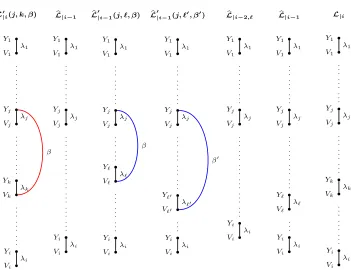
The proof of Theorem5.1 uses an inductive approach similar to the one in [37]. We postpone the complete proof to supplementary materialD.
6
Tight Security Bound of
CLRW2
Based on the tools we developed in section4and5, we now show that theCLRW2
construction achieves security up to the query complexity approximately 23n/4. Given Mennink’s attack [29] (see supplementary material B) in roughly these many queries we can conclude that the bound is tight.
Theorem 6.1. Let κ, τ, n ∈N and > 0. Let E ∈BPerm(κ, n), and let H be an ({0,1}τ,{0,1}n, )-AXU hash function family. Consider
CLRW2[E,H] :{0,1}2κ× H2× {0,1}τ× {0,1}n → {0,1}n.
Forq≤2n−2 andt >0, the TSPRP security ofCLRW2[E,H]against
A(q, t)is
given by
AdvtsprpCLRW2[E,H](q, t)≤2AdvsprpE (q, t0) +∆,
where t0 = c(t +qtH), tH being the time complexity for computing the hash function H,c >0 is a constant depending upon the computation model, and
∆≤2q21.5+9q 42 2n +
32q4 22n +
13q4 23n + 2q
22+2q2
22n. (10)
Corollary 6.1. For= 1
2n, we have
AdvtsprpCLRW2[E,H](q, t)≤2AdvsprpE (q, t0) +54q 4
23n +
2q2 23n/2 +
4q2
22n. (11)
Specifically, the advantage bound is meaningful up to q≈234n−1.43 queries. The proof of Theorem 6.1 employs the Expectation method coupled with an adaptation of (2n/2q, q4/23n)-restricted mirror theory [37] in tweakable
permu-tation settings. While our use of mirror theory is somewhat inspired by its recent use in [29], in contrast to [29], we apply a modified version of mirror theory and that too for a restricted subset of queries. The complete proof of Theorem6.1is given in the remainder of this section.
6.1 Initial Step
Consider the instantiationCLRW2[EK1, EK2,H1,H2] ofCLRW2[E,H], whereK1,
K2, H1, H2 are independent and (K1,K2)←$({0,1}κ)2, (H1,H2)←$H2. As the first step, we switch to the information-theoretic setting, i.e. we replace (EK1, EK2) with (Π1,Π2)←$Perm(n)2. For the sake of simplicity, we write the modified in-stantiationCLRW2[Π1,Π2,H1,H2] as CLRW2, i.e. without any parametrization. This switching is done via a standard hybrid argument that incurs a cost of 2AdvsprpE (q, t0) wheret0=O(t+qtH). Thus, we have
AdvtsprpCLRW2[E,H](q, t)≤2AdvsprpE (q, t0) +AdvtsprpCLRW2(q). (12) So, in Eq. (12), we have to give an upper bound onAdvtsprpCLRW2(q). At this point, we are in the information-theoretic setting. In other words, we consider com-putationally unbounded distinguisherA. Without loss of generality, we assume that A is deterministic and non-trivial. Under this setup, we are now ready to apply the expectation method.
6.2 Oracle Description
The two oracles of interest are: O1, the real oracle, that implements CLRW2; and, O0, the ideal oracle, that implements Πe←$BPerm(τ, n). We consider an
extended version of these oracles, the one in which they release some additional information. We use notations analogously as given in Figure3.1to describe the transcript generated byA’s interaction with its oracle.
Description of the real oracle, O1: The real oracle O1 faithfully runs
CLRW2. We denote the transcript random variable generated byA’s interaction withO1 by the usual notationΘ1, which is a 10-aryq-tuple
(Tq,Mq,Cq,Xq,Yq,Vq,Uq, λq,H1,H2),
– Ti:i-th tweak value,Mi:i-th plaintext value,Ci:i-th ciphertext value
whereCq =CLRW2(Tq,Mq). At the end of the query-response phaseO
1releases some additional information (Xq,Yq,Vq,Uq, λq,H1,H2), where for alli∈[q]:
– (Xi,Yi):i-th input-output pair forΠ1,
– (Vi,Ui):i-th input-output pair forΠ2,
– λi:i-th internal masking,H1,H2: the hash keys.
Note that Xq, Uq, and λq are completely determined by the hash keys H1,H2, and the initial transcript (Tq,Mq,Cq). But, we include them anyhow to ease the analysis.
Description of the ideal oracle, O0: The ideal oracle O0 has access toΠe.
SinceO1releases some additional information,O0must generate these values as well. The ideal transcript random variableΘ0is also a 10-aryq-tuple
(Tq,Mq,Cq,Xq,Yq,Vq,Uq, λq,H1,H2),
defined below. Note that we use the same notation to represent the variables of transcripts in the both world. However, the probability distributions of the these would be determined from their definitions. The initial transcript consists of (Tq,Mq,Cq), where for alli∈[q]:
– Ti:i-th tweak value,Mi:i-th plaintext value,Ci:i-th ciphertext value, where Cq =
e
Π(Tq,Mq). Once the query-response phase is overO0 first samples
(H1,H2)←$H2 and computesXq,Uq, λq, where for alli∈[q]:
– Xi:=H1(Ti)⊕Mi,Ui:=H2(Ti)⊕Ci,λi:=H1(Ti)⊕H2(Ti).
This means thatXq,Uq, andλq are defined honestly. Given the partial transcript
Θ00:= (Tq,Mq,Cq,Xq,Uq, λq,H1,H2) we wish to characterize the hash keyH:= (H1,H2) as good or bad. We writeHbadfor the set of bad hash keys, andHgood= H2\ Hbad. We say that a hash keyH∈ Hbad(or His bad) if and only if one of the following predicates is true:
1. H1: ∃∗i, j∈[q] such that Xi =Xj∧Ui=Uj. 2. H2: ∃∗i, j∈[q] such that Xi =Xj∧λ
i=λj.
3. H3: ∃∗i, j∈[q] such that Ui=Uj∧λ
i=λj.
4. H4: ∃∗i, j, k, `∈[q] such thatXi =Xj∧Uj =Uk∧Xk=X`. 5. H5: ∃∗i, j, k, `∈[q] such thatUi=Uj∧Xj=Xk∧Uk =U`. 6. H6: ∃k≥2n/2q,∃∗i1, i2, . . . , ik ∈[q] such that Xi1 =· · ·=Xik. 7. H7: ∃k≥2n/2q,∃∗i
1, i2, . . . , ik ∈[q] such that Ui1 =· · ·=Uik.
Case 1.His bad: If the hash keyHis bad, thenYq andVq values are sampled
degenerately as Yi = Vi = 0 for all i ∈ [q]. It means that we sample without maintaining any specific conditions, which may lead to inconsistencies.
Case 2. H is good: To characterize the transcript corresponding to a good
G(Xq,Uq) arising due toH∈ H
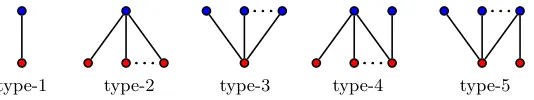
good. Lemma6.1and Figure6.1characterizes the different types of possible components in G(Xq,Uq). Note that, type-2, type-3,
type-4, and type-5 graphs are the same as configuration (A), (D), (C), and (F) of Figure3.3, for≥4 edges. These graphs are considered as bad in [29], whereas we allow such components.
type-1
. . . . . . . . .
type-2
. . .. . .. . .
type-3
. . . . . . . . .
type-4
. . . . . . . . .
type-5
Fig. 6.1: Enumerating all possible types of components of a transcript graph corre-sponding to a good hash key: type-1 is the only possible component of size = 1 edge; type-2 and type-3 are X-? and U-? components, respectively; type-4 and type-5 are the only possible components that are not isolated or star (can have degree 2 vertices in bothX andU).
Lemma 6.1. The transcript graph G corresponding to(Xq,Uq) generated by a
good hash keyHhas the following properties: 1. G is simple, acyclic and has no isolated vertices.
2. G has no two adjacent edgesiandj such thatλi⊕λj= 0.
3. G has no component of size>2n/2q edges.
4. G has no component such that it has2 distinct degree2 vertices inX orU. In fact the all possible types of components of G are enumerated in Figure6.1.
The proof of Lemma 6.1 is elementary and given in supplementary material E for the sake of completeness.
In what follows, we describe the sampling of Yq and Vq when H ∈ Hgood.
We collect the indices i ∈[q] corresponding to the edges in all type-1, type-2, type-3, type-4, and type-5 components, in the index setsI1,I2,I3,I4, andI5, respectively. Clearly, the five sets are disjoint, and [q] =I1t I2t I3t I4t I5. LetI=I1t I2t I3. Consider the system of equation
L={Yi⊕Vi=λi : i∈ I},
whereYi=Yj(res.Vi=Vj) if and only ifXi=Xj(res.Ui=Uj) for alli, j∈[q].
The solution set ofLis precisely the set
S={(yI, vI) :yI !XI∧vI!UI∧yI⊕vI =λI}. Given these definitions, the ideal oracleO0samples (Yq,Vq) as follows:
– (YI,VI)←$S, i.e. O0uniformly samples one valid assignment from the set of all valid assignments.
– LetG \ I denote the subgraph ofG after the removal of edges and vertices corresponding toi∈ I. For each componentC ofG \ I:
• Suppose (Xi,Ui)∈ C corresponds to the edge inC, where both Xi and
• For each edge (Xi0,Ui0) 6= (Xi,Ui) ∈ C, either Xi0 = Xi or Ui0 = Ui. Suppose, Xi0 =Xi. Then, Yi0 = Yi and Vi0 = Yi0 ⊕λi0. Now, suppose
Ui0 =Ui. Then, Vi0 =Vi andYi0 =Vi0⊕λi0.
At this point,Θ0= (Tq,Mq,Cq,Xq,Yq,Vq,Uq, λq,H1,H2) is completely defined. In this way we maintain both the consistency of equations of the formYi⊕Vi=λi
(as in the case of real world), and the permutation consistency within each component, whenH∈ Hgood. However, there might be collisions among Yor V
values from different components.
6.3 Definition and Analysis of Bad Transcripts
Given the description of the transcript random variable corresponding to the ideal oracle we can define the set of transcripts Ω as the set of all tuples ω = (tq, mq, cq, xq, yq, vq, uq, λq, h
1, h2), where tq ∈ ({0,1}τ)q; mq, cq, yq, vq ∈ ({0,1}n)q; (h
1, h2)∈ H2;xq =h1(tq)⊕mq;uq =h2(tq)⊕cq;λq =h1(tq)⊕h2(tq); and (tq, mq)
!(tq, cq).
Our bad transcript definition is inspired by two requirements:
1. Eliminate all xq, uq, and λq tuples such that both yq and vq are trivially
restricted by way of linear dependence. For example, consider the condition H2. This leads to yi =yj, which would imply vi =yi⊕λi =yj⊕λj =vj.
Assumingi > j,vi is trivially restricted (=vj) by way of linear dependence.
This may lead touq 6
!vq as u
i may not be equal touj.
2. Eliminate all xq,uq,yq,vq tuples such thatxq 6
!yq oruq 6
!vq.
Among the two, requirement 2 is trivial asxq!yq anduq !vq is always true for real world transcript. Requirement 1 is more of a technical one that helps in the ideal world sampling ofyq andvq.
Bad Transcript Definition: We first define certain transcripts as bad
de-pending upon the characterization of hash keys. Inspired by the ideal world description, we say that a hash key (h1, h2) ∈ Hbad (or (h1, h2) is bad) if and only if the following predicate is true:
H1∨H2∨H3∨H4∨H5∨H6∨H7.
We say thatω ishash induced bad transcript, if (h1, h2)∈ Hbad. We write this event asBAD-HASH, and by a slight abuse of notations,3 we have
BAD-HASH= 7
[
i=1
Hi. (13)
This takes care of the first requirement. For the second one we have to enumerate all the conditions which might lead to xq !6 yq or uq !6 vq. Since we sample degenerately when the hash key is bad, the transcript is trivially inconsistent in this case. For good hash keys, if xi = xj (or ui = uj) then we always have
3
yi = yj (res. vi =vj); hence the inconsistency won’t arise. So, given that the
hash key is good, we say thatωissampling induced bad transcript, if one of the following conditions is true:
for someα∈[5] andβ ∈ {α, . . . ,5}, we have
– Ycollαβ: ∃i∈ Iα, j∈ Iβ, such thatxi6=xj∧yi =yj, and – Vcollαβ: ∃i∈ Iα, j∈ Iβ, such thatui6=uj∧vi =vj,
whereIi is defined as before in section6.2. By varyingαandβ over all possible
values, we get all 30 conditions which might lead toxq 6
!yq oruq 6
!vq. Here
we remark that some of these 30 conditions are never satisfied due to the sam-pling mechanism prescribed in section6.2. These areYcoll11,Ycoll12,Ycoll13, Ycoll22, Ycoll23, Ycoll33, Vcoll11,Vcoll12, Vcoll13, Vcoll22, Vcoll23, and Vcoll33. We listed them here only for the sake of completeness. We write the combined event that one of the 30 conditions hold as BAD-SAMP. Again by an abuse of notations, we have
BAD-SAMP= [
α∈[5],β∈{α,...,5}
(Ycollαβ∪Vcollαβ). (14)
Finally, a transcript ω is called bad, i.e. ω ∈ Ωbad, if it is either a hash or a sampling induced bad transcript. All other transcripts are called good. It is easy to see that all good transcripts are attainable (as required in the H-coefficient technique or the expectation method).
Bad Transcript Analysis: We analyze the probability of realizing a bad transcript in the ideal world. By definition, this is possible if and only if one of BAD-HASHorBAD-SAMPoccurs. So, we have
bad= Pr [Θ0∈Ωbad] = Pr Θ0
[BAD-HASH∪BAD-SAMP]
≤Pr
Θ0[BAD-HASH]
| {z }
hash
+ Pr
Θ0[BAD-SAMP]
| {z }
samp
. (15)
Lemma 6.2 upper boundshash to 2q22+ 2q21.5+ 16q42−2n and Lemma 6.3 upper boundssamp to 9q422−n. Substituting these values in Eq. (15), we get
bad≤2q22+ 2q21.5+ 16q4
22n +
9q42
2n . (16)
Lemma 6.2. hash≤2q22+ 2q21.5+16q 4 22n .
Proof. Using Eq. (13) and (15), we have
hash= Pr [H1∪H2∪H3∪H4∪H5∪H6∪H7]≤ 7
X
i=1 Pr [Hi].
H1is true if for some distincti, jboth Xi=Xj, andUi=Uj. NowTi=Tj =⇒
fixedi, j we get an upper bound of 2 asHis-AXU, and we have at most q
2
pairs ofi, j. Thus, Pr [H1]≤ q2
2. Following a similar line of argument one can bound Pr [H2]≤ q2
2 and Pr [H 3]≤ q2
2.
In the remaining, we bound the probability ofH4andH6, while the probability ofH5andH7can be bounded analogously. For any functionf :{0,1}τ ∈ {0,1}n,
letf0 :{0,1}τ× {0,1}n → {0,1}n be defined as f0(t, m) =f(t)⊕m. SoXi =
H01(Ti,Mi), and Ui =H02(Ti,Ci), for all i ∈ [q]. It is easy to see that H0b is -universal ifHb is-AXU forb∈[2]. Using the renewed description,H4is true if for some distinct i, j, k, `,
H01(Ti,Mi) =H01(Tj,Mj)∧H02(Tj,Cj) =H02(Tk,Ck)∧H01(Tk,Mk) =H01(T`,M`). Since (ti, mi)6= (tj, mj) and (ti, ci)6= (tj, cj) for distinct iand j, we can apply
the alternating collisions lemma of Lemma4.1to get Pr [H4]≤q21.5. ForH6, we have
Xi1=Xi2 =· · ·=Xik,
where k≥2n/2q. Since, (tij, mij)6= (til, mil) for allj6=l, we can apply Corol-lary4.1 witha= 2n/2qto get Pr [H6]≤8q4
22n. ut
Lemma 6.3. samp≤ 9q 42 2n .
Proof. Using Eq. (14) and (15), we have
samp= Pr
[
α∈[5],β∈{α,...,5}
(Ycollαβ∪Vcollαβ)
≤ X
α∈[5]
X
β∈{α,...,5}
Pr [Ycollαβ] + Pr [Vcollαβ]
.
We bound the probabilities of the events on the right hand side in groups as given below:
1. BoundingP
α∈[3],β∈{α,...,3}Pr [Ycollαβ] + Pr [Vcollαβ]: Recall that the
sam-pling of Y and V values is always done consistently for indices belonging to I =I1t I2t I3. Hence,
X
α∈[3],β∈{α,...,3}
Pr [Ycollαβ] + Pr [Vcollαβ] = 0, (17)
2. BoundingP
α∈[3],β∈{4,5}Pr [Ycollαβ] + Pr [Vcollαβ]: Let’s consider the event
Ycoll14, which translates to there exist indices i ∈ I1 and j ∈ I4 such that
Xi6=Xj∧Yi=Yj. Since j∈ I4, there must exist k, `∈ I4\ {j}, such that one of the following happens
Uj=Uk∧Xk =X`
Xj=Xk∧Uj=U`.
We analyze the first case, while the other two cases can be similarly bounded. To bound the probability ofYcoll14, we can thus look at the joint event
E: ∃i∈ I1,∃∗j, k, `∈ I4, such thatYi=Yj∧Xj=Xk∧Uk =U`.
Note that the event Yi =Yj is independent ofXj =Xk∧Uk =U`, as bothYi
andYj are sampled independent of the hash key. Thus, we get
Pr [E] = Pr [∃i∈ I1,∃∗j, k, `∈ I4, such thatYi=Yj∧Xj=Xk∧Uk =U`]
≤ X
i∈I1
X
j<k<`∈I4
Pr [Yi=Yj]×Pr [Xj =Xk∧Uk=U`]
≤q
q 3
2 2n,
where the last inequality follows from the uniform randomness of Yj and the AXU property ofH1andH2. The probability of the other two cases are similarly bounded toq 3q22n, whence we get
Pr [Ycoll14]≤3q
q
3
2
2n.
We can bound the probabilities of Ycoll24, Ycoll34, Ycollα5, Vcollα4, and Vcollα5, forα∈[3], in a similar manner as in the case ofYcoll14. So, we skip the argumentation for these cases, and summarize the probability for this group as
X
α∈[3],β∈{4,5}
Pr [Ycollαβ] + Pr [Vcollαβ]≤
6q42
2n . (18)
3. BoundingP
α∈{4,5},β∈{α,5}Pr [Ycollαβ] + Pr [Vcollαβ]: Consider the event
Ycoll44, which translates to there exists distinct indices i, j ∈ I4 such that
Xi 6=Xj∧Yi=Yj. Here asi, j∈ I4, there must existk, `∈ I4\ {j}such that one of the following happens
Xj=Xk∧Uk=U`
Uj=Uk∧Xk =X`
Xj=Xk∧Uj=U`.
The analysis of these cases is similar to 2 above. So, we skip it and provide the final bound
Pr [Ycoll44]≤3q
q
3
2
The probabilities of all the remaining events in this group can be bounded in a similar fashion.
X
α∈{4,5},β∈{α,5}
Pr [Ycollαβ] + Pr [Vcollαβ]≤
3q42
2n . (19)
The result follows by combining Eq. (17-19), followed by some algebraic
simpli-fications. ut
6.4 Good Transcript Analysis
From section 6.2, we know the types of components present in the transcript graph corresponding to a good transcript ω are exactly as in Figure 6.1. Let ω = (tq, mq, cq, xq, yq, vq, uq, λq, h
1, h2) be the good transcript at hand. From the bad transcript description of section6.3, we know that for a good transcript (tq, mq)
!(tq, cq),xq
!yq,vq
!uq, andyq⊕vq=λq.
We add some new parameters with respect toω to aid our analysis of good transcripts. For i ∈ [5], let ci(ω) and qi(ω) denote the number of components
and number of indices (corresponding to the edges), respectively of type-i in ω. Note thatq1(ω) = c1(ω), qi(ω) ≥2ci(ω) fori ∈ {2,3}, and qi(ω)≥ 3ci(ω)
for i ∈ {4,5}. Obviously, for a good transcript q = P5
i=1qi(ω). For all these
parameters, we will drop theω parametrization whenever it is understood from the context.
Interpolation probability for the real oracle: In the real oracle,
(H1,H2)←$H2,Π1 is called exactlyq1+c2+q3+ 2c4+q5−c5 times andΠ2 is called exactlyq1+q2+c3+q4−c4+ 2c5times. Thus, we have
Pr [Θ1=ω] = 1 |H|2 ×
1 (2n)
q1+c2+q3+2c4+q5−c5
× 1
(2n)
q1+q2+c3+q4−c4+2c5 . (20)
Interpolation probability for the ideal oracle: In the ideal oracle,
the sampling is done in parts:
I. Πe sampling: Let (t01, t20,· · ·, t0r) denote the tuple of distinct tweaks intq, and
for alli∈[r], letai=µ(tq, t0i), i.e.r≤q and Pr
i=1ai=q. Then, we have
PrhΠe(tq, mq) =cq i
≤Qr 1 i=1(2n)ai
.
II. Hash key sampling: The hash keys are sampled uniformly from H2, i.e. Pr [(H1,H2) = (h1, h2)] =|H|12.
III. Internal variables sampling: The internal variables Yq and Vq are sampled
in two stages.
(A). type-1, type-2 and type-3 sampling: Recall the sets I1, I2, andI3, from section6.3. Consider the system of equation
Let (λ01, λ02,· · ·, λ0s) denote the tuple of distinct elements inλI, and for alli∈[s], let bi =µ(λI, λ0i). From Figure6.1 we know that Lis
cycle-free and non-degenerate. Further,ξmax(L)≤2n/2q, since the transcript is good. So, we can apply Theorem5.1to get a lower bound on the the number of valid solutions,|S| for L. Using the fact that (YI,VI)←$S, and Theorem5.1, we have
Pr
(YI,VI) = (yI, vI)
≤
Qs i=1(2
n) bi ζ(ω)(2n)
q1+c2+q3(2
n)
q1+q2+c3 ,
where
ζ(ω) = 1−13q 4
23n −
2q2 22n −
c2+c3
X
i=1 ηc21+i
!
4q2 22n
!
,
(B). type-4, and type-5 sampling: For the remaining indices, one value is sam-pled uniformly for each of the components, i.e. we have
PrhY[q]\I,V[q]\I=y[q]\I, v[q]\Ii= 1 (2n)c4+c5.
By combiningI,II,III, and rearranging the terms, we have
Pr [Θ0=ω]≤ 1 |H|2×
1 ζ(ω)×
Qs i=1(2
n) bi
Qr
i=1(2n)ai(2
n) p1(2
n) p2(2
n)c4+c5, (21)
wherep1=q1+c2+q3, and p2=q1+q2+c3.
6.5 Ratio of Interpolation Probabilities
On dividing Eq. (20) by Eq. (21), and simplifying the expression, we get
Pr [Θ1=ω] Pr [Θ0=ω]
≥ζ(ω)·
Qr i=1(2
n) ai
Qs
i=1(2n)bi(2
n−p
1−c4)c4+q5−c5(2
n−p
2−c5)q4−c4+c5 1
≥ζ(ω)·
Qr
i=1(2n)di
Qr
i=1(2n−di)ai−di
Qs
i=1(2n)bi(2
n−p1−c4)
c4+q5−c5(2
n−p2−c5)
q4−c4+c5 2
≥ζ(ω)·
Qr
i=1(2n−di)ai−di (2n−p
1−c4)c4+q5−c5(2
n−p
2−c5)q4−c4+c5
)
A
3
≥ζ(ω). (22)
At inequality 1, we rewrite the numerator such that di = µ(tI, t0i) for i ∈ [r].
Further, r ≥ s, as number of distinct internal masking values is at most the number of distinct tweaks, andbtI compresses tobλI. So using Proposition1, we
can justify inequality 2. At inequality 2, fori∈ {2,3,4,5},ci(ω)>0 if and only
ifr≥2. Also,di≤c1+c2+c3≤p1+c4anddi≤p2+c5 fori∈[r]. Similarly,
Pr
i=1ai−di=q4+q5. Thus, A satisfies the conditions given in Proposition2, and henceA≥1. This justifies inequality 3.
We defineratio:Ω→[0,∞) by the mapping
ratio(ω) = 1−ζ(ω).
Clearly ratio is non-negative and the ratio of real to ideal interpolation proba-bilities is at least 1−ratio(ω) (using Eq. (22)). Thus, we can use Lemma 2.1to get
AdvtsprpCLRW2(q)≤ 2q 2
22n +
13q4 23n +
4q2 22nEx
"c2+c3
X
i=1 η2c1+i
#
+bad. (23)
Let ∼1 (res. ∼2) be an equivalence relation over [q], such that α ∼1 β (res. α∼2 β) if and only if Xα=Xβ (res.Uα=Uβ). Now, each ηi random variable
denotes the cardinality of some non-singleton equivalence class of [q] with respect to either ∼1 or ∼2. Let P1
1, . . . ,Pr1 and P12, . . . ,Ps2 denote the non-singleton
equivalence classes of [q] with respect to ∼1 and ∼2, respectively. Further, for i∈[r] andj∈[s], letνi=|Pi1|andνj0 =|Pj2|. Then, we have
Ex "c2+c3
X
i=1 ηc2
1+i
#
≤Ex
r X
j=1 νj2
+Ex " s
X
k=1 νk02
#
≤4q2. (24)
where the first inequality follows from the fact thatH1andH2are independently sampled, and the second inequality follows from Lemma 4.3 and the fact that
H1,H2←$H. Theorem 6.1follows from Eq. (12), (16), (23)-(24). ut
7
Further Discussion
In this paper, our chief contribution is a tight (up to a logarithmic factor) security bound for the cascaded LRW2 tweakable block cipher. We developed two new tools: first, we provide a probabilistic result, called alternating collisions (events) lemma, that gives improved bounds for some special collision events, that are encountered frequently in BBB security analysis. Second, we adapt a restricted variant of mirror theory in tweakable permutations setting.
7.1 Applications of Alternating Events Lemma and Mirror Theory
The combination of alternating events lemma and mirror theory seem to have some nice applications. Here, we give some applications based on the Double-block Hash-then-Sum (or DbHtS) paradigm by Datta et al. [42]. The DbHtS
paradigm is a variable input length pseudorandom function or PRF construction, based on a block cipherE and a hash functionH, which is defined as:
∀(k2, h, m)∈ {0,1}2κ× H × {0,1}∗,
DbHtS[E,H](k2, h, m) =λ=E
where{0,1}∗ denotes the set of all bit strings, and (x, u) =h(m).
PRF Security: Let F be a keyed function family from {0,1}∗ to {0,1}n
indexed by the key space{0,1}κ. We define the PRF-advantage of an adversary
A againstF as,
AdvprfF (A) =
Pr K
AFK= 1−Pr
Γ
AΓ= 1
,
whereK←${0,1}κ, andΓis a uniform random function chosen from the set of all
functions from{0,1}∗ to{0,1}n. The PRF security of F against any adversary
classA(q, t) is defined analogously to SPRP and TSPRP security given in section
2.3.
Application 1:DbHtS-p— As a first application, we relax theDbHtS construc-tion toDbHtS-p, where the hash functionhis made up of independent universal hash functionsh1 andh2, such that h(m) = (h1(m), h2(m)). This construction was also analyzed in [51], though they showed security up toq22n/3.
We show thatDbHtS-pachieves higher security (i.e. security up toq23n/4). Further, the attack by Leurent et al. [53] in roughly 23n/4queries, seems to apply toDbHtS-pfor algebraic hash functions. Thus, our bound is tight.
Theorem 7.1. For q ≤ 2n−2 and t > 0, the PRF security of DbHtS-p[E,H] against A(q, t)is given by
AdvprfDbHtS-p[E,H](q, t)≤2AdvprpE (q, t0) +∆,
where t0 = c(t +qtH), tH being the time complexity for computing the hash function H,c >0 is a constant depending upon the computation model, and
∆≤2q21.5+9q 42 2n +
32q4 22n +
13q4 23n +q
22+q2 2n +
2q2
22n. (25)
Note that the PRP security game is similar to SPRP, except that the adversary is not given inverse access to the oracle. The proof of Theorem 7.1 is given in supplementary materialF.
Application 2:DbHtS-f— TheDbHtS-fis another relaxation of DbHtS, where the hash function h is made up of independent universal hash functions h1 and h2, and the finalization is done via keyed functions Fk1 and Fk2, i.e.,
DbHtS-f(m) = λ = Fk1(x)⊕Fk2(u), where x = h1(m) and u = h2(m). We
show that DbHtS-fis secure up toq23n/4.
Theorem 7.2. For q ≤ 2n−2 and t > 0, the PRF security of DbHtS-f[F,H] against A(q, t)is given by