Towards End-to-End Acoustic Localization Using Deep Learning: From Audio Signal to Source Position Coordinates

Towards End-to-End Acoustic Localization using

Deep Learning: from Audio Signal to Source Position

Coordinates

Juan Manuel Vera-Diaz, Daniel Pizarro and Javier Macias-Guarasa ∗

1

2

3

4

5

6

7

8

9

10

11

12

13

14

DepartmentofElectronics,UniversityofAlcalá,CampusUniversitarios/n,28805,AlcaládeHenares,Madrid, Spain. [email protected], [email protected], [email protected]

* Correspondence: [email protected]; Tel.: +34-91-885-6918

Abstract: This paper presents a novel approach for indoor acoustic source localization using microphone arrays and based on a Convolutional Neural Network (CNN). The proposed solution is, to the best of our knowledge, the first published work in which the CNN is designed to directly estimate the three dimensional position of an acoustic source, using the raw audio signal as the input information avoiding the use of hand crafted audio features. Given the limited amount of available localization data, we propose in this paper a training strategy based on two steps. We first train our network using semi-synthetic data, generated from close talk speech recordings, and where we simulate the time delays and distortion suffered in the signal that propagates from the source to the array of microphones. We then fine tune this network using a small amount of real d ata. Our experimental results show that this strategy is able to produce networks that significantly improve existing localization methods based on SRP-PHATstrategies. In addition, our experiments show that our CNN method exhibits better resistance against varying gender of the speaker and different window sizes compared with the other methods.

Keywords: acoustic source localization; microphone arrays; deep learning; convolutional neural networks

15

1. Introduction 16

The development and scientific research in advanced perceptual systems has notably grown 17

during the last decades, and has experimented a tremendous rise in the last years due to the 18

availability of increasingly sophisticated sensors, the use of computing nodes with higher and higher 19

computational power, and the advent of powerful algorithmic strategies based on deep learning 20

(all of them actually entering the mass consumer market). The aim of perceptual systems is to 21

automatically analyze complex and rich information taken from different sensors, in order to obtain 22

refined information on the sensed environment and the activities being carried out within them. The 23

scientific works in these environments, cover research areas from basic sensor technologies, to signal 24

processing and pattern recognition, and open the path to the idea of systems able to analyze human 25

activities, providing them with advanced interaction capabilities and services.. 26

In this context, localization of humans (being the mostinterestingelement for perceptual systems) 27

is a fundamental task that needs to be addressed so that the systems can actually start to provide higher 28

level information on the activities being carried out. Without a precise localization, further advanced 29

interaction between humans and their physical environment cannot be carried out successfully. 30

The scientific community has devoted a huge amount of effort to build robust and reliable indoor 31

localization systems, based on different sensors [1–3]. Non-invasive technologies are preferred in this 32

context, so that no electronic or passive devices need to be carried by humans for localization. The two 33

non-invasive technologies that have been mainly used in indoor localization are those based on video 34

systems and acoustic sensors. 35

This paper focuses on audio-based localization, with no previous assumptions on the acoustic 36

signal characteristics nor in the physical environment, apart from the fact that unknown wide-band 37

audio sources (e.g. human voice) are captured by a set of microphone arrays placed in known positions. 38

The main objective of the paper is to directly use the signals captured by the microphone arrays to 39

automatically obtain the position of the the acoustic source detected in the given environment. 40

Even though there are a lot of proposals in this area, Acoustic Source Localization (ASL) is still 41

a hot research topic. This paper proposes a convolutional neural network (CNN) architecture that 42

is trained end-to-end to solve the acoustic localization problem. To our knowledge, this is the first 43

work in the literature that does not provide the network with feature vectors extracted from the speech 44

signals, but directly uses the speech signal. Avoiding hand crafted features has been proved to increase 45

the accuracy of classification and regression methods based on convolutional neural networks in other 46

fields, such as in computer vision [4,5]. 47

Our proposal is evaluated using both semi-synthetic and real data, outperforming traditional 48

solutions based on Steered Response Power (SRP) [6], that are still the basis of state-of-the-art 49

systems [7–10]. 50

The rest of the paper is organized as follows. In Section2a review study of the state-of-the-art in 51

acoustic source localization with special emphasis on the use of deep learning approaches. Section3 52

describes the CNN based proposal, with details on the training and fine tuning strategies. The 53

experimental work is detailed in Section4, and Section5summarizes the main conclusions and 54

contributions of the paper and gives some ideas for future work. 55

2. State of the Art 56

Many approaches exist in the literature to address the acoustic source localization (ASL) problem. 57

According to the classical literature review in this topic, these approaches can be broadly divided in 58

three categories [11,12]: time delay based, beamforming based, and high-resolution spectral-estimation 59

based methods. This taxonomy relies in the fact that ASL has been traditionally considered a signal 60

processing problem based on the definition of a signal propagation model [11–19], but, more recently, 61

the range of proposals in the literature also considered strategies based on exploiting optimization 62

techniques and mathematical properties of related measurements [20–24], and also using machine 63

learning strategies [25–27], aimed at obtaining a direct mapping from specific features to source 64

locations [28], area in which deep learning approaches are starting to be applied and that will be 65

further described later in this section. 66

Time delay based methods (also referred to asindirect methods), compute the time difference of 67

arrivals (TDOAs) across various combinations of pairs of spatially separated microphones, usually 68

using the Generalized Correlation Function (GCC) [13]. In a second step, the TDOAs are combined 69

with knowledge of the microphones’ positions to generate a position estimation [11,29]. 70

Beamforming based techniques [12,15,19,30] attempt to estimate the position of the source, 71

optimizing a spatial statistic associated with each position, such as in the Steered Response Power 72

(SRP) approach, in which the statistic is based on the signal power received when the microphone 73

array is steered in the direction of a specific location. SRP-PHAT is a widely used algorithm for 74

speaker localization based on beamforming that was first proposed in [6]1. It combines the robustness 75

of the SRP approach with the Phase Transform (PHAT) filtering, which increases the robustness 76

of the algorithm to signal and room conditions, making it an ideal strategy for realistic speaker 77

localization systems [16,17,32–34]. Other beamforming based methods such as the Minimum Variance 78

Distortionless Response (MVDR) [18], exhibits problems when facing reverberant environments, 79

because it introduces a new trade-off between dereverberation and noise reduction. 80

In what respect to spectral estimation based methods, the multiple signal classification algorithm 81

(MUSIC) [35], has been widely used, but these methods, in general, tend to be less robust than 82

beamforming methods [12], as they assume incoherent signals and are very sensitive to small modeling 83

errors. 84

In the past few years, deep learning approaches [36] have taken the lead in different signal 85

processing and machine learning fields, such as computer vision [37,38] and speech recognition [39– 86

41], and, in general, in any area in which complex relationships between observed signals and the 87

underlying processes generating them need to be discovered. 88

The idea of using neural networks for ASL is not new. Back in the early nineties and the first 89

decade of the current century, works such as [25,42,43] proposed the use of neural network techniques 90

in this area. However an evaluation on realistic and extensive data sets was not viable at this time, and 91

the proposals were somehow limited in scope. 92

With the advent and huge increase on applications of deep neural networks in all areas of machine 93

learning, and mainly due to the sophisticated capabilities and more careful implementation details 94

of network architectures and the availability of advanced hardware architectures with increased 95

computational capacity, promising works have been proposed also for ASL [44–58]. 96

The main differences between the different proposals using neural networks for ASL reside in the 97

architectures, input features, the network output (target), and the experimental setup (using real or 98

simulated data). 99

Regarding the information given to the neural network, we can find several works using features 100

physically related to the ASL problem. Some of the proposals use features derived from the GCC 101

or related functions, which actually make sense as these correlation function is closely related to 102

the TDOAs which are used in traditional methods to generate position estimations. The published 103

works use either the GCC coefficients directly [50], features derived from them [45,55] or from the 104

correlation matrix [47,49], or even combined with others, such as cepstral coefficients [53]. Other works 105

are focused in exploiting binaural cues [44,46], features derived from convolving the spectrum with 106

head related impulse responses [58] or even narrowband SRP values [56]. The latter approach goes 107

one step further from correlation related values, as the SRP function actually integrates multiple GCC 108

estimations in such a way that acoustic energy maps can be easily generated from it. 109

Opposed to the previously described works using refined features directly related to the 110

localization problem, we can also find others using frequency domain features directly [48,52], in 111

some cases generated from spectrograms of general time-frequency representations [51,54]. These 112

approaches represent a step forward compared with the previous ones, as they give the network the 113

responsibility of automatically learn the relationship between spectral cues and the location related 114

information [57] kind of combines both strategies, as they use spectral features but calculating them 115

in a cross-spectral fashion, that is, combining the values from all the available microphones in the 116

so-called Cross Spectral Map (CSM). 117

In none of the referenced works, the authors try to make use of the raw acoustic signal directly, 118

and we are interested in evaluating the capabilities of CNN architectures in directly exploiting this raw 119

input information. 120

In what respect to the estimation target, most of the works are oriented towards estimating the 121

Direction of Arrival (DOA) of the acoustic sources [45,50,51,55,56], or DOA related measurements 122

such as azimuth angle [44,46,48], elevation angle [58], or position bearing+range [53]. Some of the 123

proposals pose the problem not as a direct estimation (regression) but as a classification problem among 124

a predefined set of possible position related values [47–49,52,54] (azimuth, positions in a predefined 125

grid, etc.). Works with a very different target try to estimate acleanacoustic source map [57] or learn 126

time-frequency masks as a preprocessing stage prior to ASL [59]. 127

In none of the referenced works the authors try to directly estimate the coordinate values of the 128

acoustic sources, and, again, we are interested in evaluating the capabilities of CNN architectures to 129

Finally, in what respect to the experimental setup, most works use simulated data either for 131

training or for training and testing [44–52,54–59], usually by convolving clean (anechoic) speech with 132

impulse responses (room, head related, or DOA related (azimuth, elevation)). Only some of them 133

actually face real recordings [44,45,53,55,56], which in our opinion is a must to be able to assess the 134

actual impact of the proposals in real conditions. 135

So, in this paper we describe, for the first time in the literature to the best of our knowledge, a 136

CNN architecture in which we directly exploit the raw acoustic signal to be provided to the neural 137

network, with the objective of directly estimating the three dimensional position of an acoustic source 138

in a given environment. This is the reason why we refer to this strategy as end-to-end, considering the 139

full coverage of the ASL problem. The proposal has been tested on both semi-synthetic and real data 140

from a publicly available database. 141

3. System Description 142

3.1. Problem Statement 143

Our system obtains the position of an acoustic source from the audio signals recorded by an array 144

ofMmicrophones. Given a reference coordinate origin, the source position is defined with the 3D 145

coordinate vectors= sx sy sz>. The microphones positions are known and they are defined with 146

coordinate vectorsmi = mi,x mi,y mi,z >

withi=1, . . . ,M. The audio signal captured from theith 147

microphone is denoted byxi(t). This signal is discretized with a sampling frequency fs and is defined 148

withxi[n]. We assume for simplicity thatxi[n]is of finite-length withNsamples. This corresponds to 149

a small window of audio with durationws =N/fs, which is a design parameter in our system. We 150

denote asxithe vector containing all time samples of the signal: 151

xi=

xi[0] . . . xi[N−1] >

. (1)

The problem we seek to solve is to find the following regression functionf:

s= f(x1, . . . ,xN,m1, . . . ,mM), (2) that obtains the speaker position given the signals recorded from the microphones.

152

In classical simplified approaches, f is found by assuming that signals received from different 153

microphones mainly differ by a delay that depends on the relative position of the source with respect 154

to the microphones. However, this assumption breaks in environments where the signal suffers from 155

random noise and distortion, such as multi-path signals or microphone non-linear response. 156

Due to the aforementioned effects, and the random nature of the audio signal, the regression 157

function of equation (2) cannot be estimated analytically. We present in this paper a learning approach 158

for directly obtainingf using Deep Learning. We representf using a Convolutional Neural Network 159

(CNN) which is learned end-to-end from the microphone signals. In our system we assume that 160

microphones positions are fixed. We thus drop the requirement of knowing the microphone’s position 161

from equation (2) which will be implicitly learned by our network with the following regression 162

problem: 163

s= fnet(x1, . . . ,xM), (3)

where fnetdenotes the function that we represent using the CNN and whose topology is described 164

next. 165

3.2. Network Topology 166

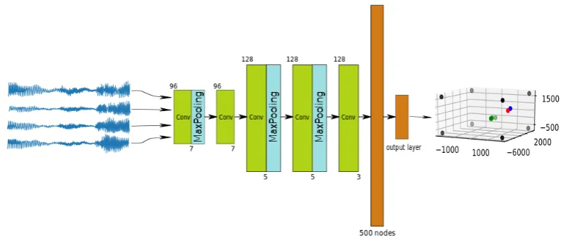
The topology of our neural network is shown in figure1. It is composed of five convolutional 167

are the set of windowed signals from the microphones and the network output is the estimated position 169

of the acoustic source. 170

Figure 1.Used network topology

Table (1) shows the size and amount of convolutional filters in the proposed network. We use 171

filters of size 7 (layers 1 and 2), size 5 (layers 3 and 4) and size 3 (layer 5). The number of filters is 96 172

in the first two convolutional layers and 128 in the rest. As seen in figure1, some of the layers are 173

equipped withMaxPoolingfilters with the same pool size as their corresponding convolutional filters. 174

The last two layers are fully-connected layers, one hidden with 500 nodes and the output layer. All 175

layer’s activation functions are “ReLUs” with the exception of the output layer. During training we 176

include dropout with probability 0.5 in the fully-connected layers to prevent overfitting. 177

Table 1.Network convolutional layers summary

Block Filters Kernel Convolutional block 1 96 7 Convolutional block 2 96 7 Convolutional block 3 128 5 Convolutional block 4 128 5 Convolutional block 5 128 3

3.3. Training Strategy 178

The amount of available real data that we have in our experimental setup (see Section4) will 179

be, in general, limited for training a CNN model. To cope with this problem we propose a training 180

strategy comprising two steps: 181

Step 1. Training the network with semi-synthetic data: We use close-talk speech recordings 182

and a set of randomly generated source positions to generate simulated versions of the signals 183

captured by a set of microphones that share the same geometry with the environment used in 184

real data. Additional considerations on the acoustic behavior of the target environment (specific 185

noise types, noise levels, etc.) is also taken into account to generate the data. This dataset can 186

virtually be made as big as required to train the network. 187

Step 2. Fine tuning the network with real data: We train the network on a reduced subset of the 188

database captured in the target physical environment using the weights obtained in Step 1 as 189

3.3.1. Semi-Synthetic Dataset Generation 191

In this step we extract audio signals from any available close-talk (anechoic) corpus, and use 192

them to generate semi-synthetic data. There are many available datasets suitable for this task (freely of 193

commercially distributed). Our semi-synthetic dataset can thus be made as big as required for training 194

the CNN. 195

For this task, we randomly generate position vectorsq = qx qy qz>of the acoustic source 196

using a uniform distribution that covers the physical space (room) that will be used. 197

The loss function we use to train the network is the mean squared error between the estimated 198

position given by the network (si) and the target position vector (qi). It follows the expression: 199

L(Θ) = 1 N

N

∑

|qi−si|2, (4)

whereΘrepresents the weights of the network. Equation (4) is minimized in function of the 200

unknown weights using iterative optimization based on the Stochastic Gradient Descent (SGD) 201

algorithm [60]. We finally obtain the target weightsθ ∈ Θ once a termination criterion is met in

202

the optimization. More details are given in Section4about the training algorithm. 203

In order to realistically simulate the signals received in the microphones from a given source 204

position we have to consider two main issues: 205

• Signal propagation considerations: This is affected by the impulse response of the target room. 206

Different alternatives can be used to simulate this effect, such as convolving the anechoic signals 207

with real room impulse responses such as in [47], that can be difficult to acquire for general 208

positions in big environments; or using room response simulation methods such as the image 209

method [61] used in [62] for this purpose. 210

• Acoustic noise conditions of the room and recording process conditions: These can be due to 211

additional equipment (computers, fans, air conditioning systems, etc.) present in the room, and 212

to problems in the signal acquisition setup. This can be addressed by assuming additive noise 213

conditions, and selecting a noise type and acoustic effects that should be preferably estimated in 214

the target room. 215

In our case, and regarding the first issue, we used an initial simple approach, just taking into 216

account the propagation delay from the source position to each of the microphones, that depends on 217

their relative position and the sound speed in the room. 218

We denote the number of samples we have to shift a signal to simulate the arrival delay suffered at 219

microphoneibyNsi = fs di

c where fsis the sampling frequency of the signal,diis the euclidean distance 220

between the acoustic source and theimicrophone andcis the sound speed in air (c=343m/sin a 221

room at 20Co_{). In generalN}

si is not an integer number. We thus require a way to simulate sub-sample 222

shifts in the signal. In order to implement the delayNs_i onxpc(the windowed signal ofNsamples 223

from the close-talk dataset) to obtainxiwe use the following transformation: 224

Xpc=F {xpc} xi =Ai

F−1_{XpcDs

i

, withDs_i =

1,e−j 2π_Nsi

N _,e−j 4π_Nsi

N _,· · ·_,e−j(N−1) 2π_Nsi

N

(5)

where we first transformxpcinto the frequency domainXpcusing theDiscrete Fourier Transformoperator 225

F. We then change its phase according toNsi by the phase vectorDsi and transform the signal back 226

into time domainxi, using theInverse Discrete Fourier TransformoperatorF-1. Ai is an amplitude 227

factor applied to the signal that follows a uniform random distribution, and it is different for each 228

microphone, preventing the network from being affected by amplitude differences between the signals 229

captured in different microphones (Ai ∈[0.01, 0.03]in the experimental setup described in Section4). 230

Regarding the second issue, we simulate noise and disturbances in the signals arriving to the 231

possible to those found in the real data. In order to provide an example of the methodology we follow, 233

we refer in this section to the particular case of the IDIAP room (see Section4.1.1) that will be used in 234

our real data experiments, and the Albayzin Phonetic Corpus (see Section4.1.2) that will be used for 235

synthetic data generation. 236

In the IDIAP room, a spectrogram based analysis showed that the recordings are contaminated 237

with a tone at around 25Hzin the spectrum which does not appear in anechoic conditions, probably 238

due to room equipment of electrical noise generated in the recording hardware setup. We have 239

determined that the frequency of this tone actually varies in a range between 20Hzand 30Hz. So, 240

in the synthetic data generation process, we havecontaminatedthe signals from the phonetic corpus 241

with an additive tone of a random frequency in this established range, and we have also added white 242

gaussian noise following the expression: 243

xpcnew[n] =xpc[n] +kssin(2πf0n/fs+φ0) +kηηwgn[n], (6) whereksis a scaling factor for the contaminating tone signal (similar to the tone amplitude found in 244

the target room recordings, 0.1 in our case), f0∈[20, 30]Hz,φ0∈[0,π]rad,ηwgnis a white gaussian 245

noise signal, andkηis a noise scaling factor to generate signals with a SNR which is similar to that 246

found in the target room recordings. 247

After this procedure is applied, the semi-synthetic signal data set will be ready to be used in the 248

neural network training procedure. 249

3.3.2. Fine Tuning Procedure 250

The previous step takes care of reproducing simple acoustic characteristics of the testing room 251

such as the propagation effects and the presence of specific types and levels of additive noises, but 252

there are other phenomena like multi-path and reverberation propagation which are more complex 253

to simulate. In order to introduce these acoustic behaviors of the target physical environment, our 254

proposal is to carry out a fine tuning procedure of the network model using a short amount of real 255

recorded data in the target room 256

Although there are other methods such as the one proposed in [49], where an unsupervised DNN 257

is implemented for the adaptation of parameters to unknown data, we believe that the fine tuning 258

process implemented is adequate because, in the first place, it is a supervised process with which a 259

better performance is expected to be obtained and, secondly, not all the sequences of the test data set 260

are used, so that only a few are used for the fine tuning process, saving the rest for the test phase. 261

4. Experimental Work 262

In his section we describe the datasets used in both steps of the training strategy described in 263

Section3.3, and the details associated with it. We then define the experimental setup general conditions, 264

and the error metrics used for comparing our proposal with other state-of-the-art methods and finally 265

present our experimental results, starting from the baseline performance we aim at improving. 266

4.1. Datasets 267

4.1.1. IDIAP AV16.3 Corpus: for testing and fine tuning 268

We have evaluated our proposal using the audio recordings of the AV16.3 database [63], an 269

audio-visual corpus recorded in theSmart Meeting Roomof the IDIAP research institute, in Switzerland. 270

We have also used the physical layout of this room for our semi-synthetic data generation process. 271

TheIDIAP Smart Meeting Roomis a 3.6m×8.2m×2.4mrectangular room with a rectangular table 272

centrally located and measuring 4.8m×1.2m. On the table’s surface there are two circular microphone 273

arrays of 0.1mradius, each of them composed by 8 regularly distributed microphones as shown in 274

them is considered as the origin of the coordinate reference system. A detailed description of the 276

meeting room can be found in [64]. 277

The dataset is composed by several sequences of recordings, synchronously sampled at 278

16 KHz, which a wide range of experimental conditions in the number of speakers involved 279

and their activity. Some of the available audio sequences are assigned a corresponding 280

annotation file containing the real ground truth positions (3D coordinates) of the speaker’s 281

mouth at every time frame in which that speaker was talking. The segmentation of acoustic 282

frames with speech activity was first checked manually at certain time instances by a human 283

operator in order to ensure its correctness, and later extended to cover the rest of recording 284

time by means of interpolation techniques. The frame shift resolution was defined to 285

be 40 ms. The complete dataset is fully accessible on-line at [65]. 286

(a) (b) (c)

Figure 2. (a) Simplified top view of theIDIAP Smart Meeting Room, (b) A real picture of the room extracted from a video frame, (c) Microphone setup used in this proposal

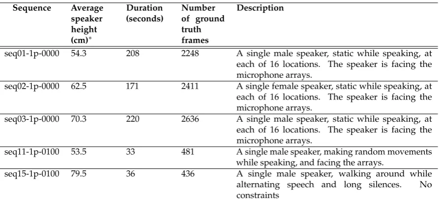
In this paper we will just focus on all the annotated sequences of this dataset featuring a single 287

speaker, whose main characteristics are shown in Table2. This allows us to directly compare our 288

performance with the state-of-the-art method presented in [20]. Note that the firsts three sequences are 289

performed by a speaker remaining static while speaking at different positions, and the last two ones 290

by a moving speaker, being all of the speakers different. We will refer to these sequences ass01,s02, 291

Table 2.IDIAP Smart Meeting Roomused sequences.

Sequence Average speaker height (cm)∗

Duration (seconds)

Number of ground truth frames

Description

seq01-1p-0000 54.3 208 2248 A single male speaker, static while speaking, at each of 16 locations. The speaker is facing the microphone arrays.

seq02-1p-0000 62.5 171 2411 A single female speaker, static while speaking, at each of 16 locations. The speaker is facing the microphone arrays.

seq03-1p-0000 70.3 220 2636 A single male speaker, static while speaking, at each of 16 locations. The speaker is facing the microphone arrays.

seq11-1p-0100 53.5 33 481 A single male speaker, making random movements while speaking, and facing the arrays.

seq15-1p-0100 79.5 36 436 A single male speaker, walking around while alternating speech and long silences. No constraints

∗_{The average speaker height is referenced to the system coordinates and refers to the speaker’s mouth height.}

4.1.2. Albayzin Phonetic Corpus: for Semi-Synthetic Dataset Generation 293

The Albayzin Phonetic Corpus [66] consists of 3 sub-corpora of 16 kHz 16 bits signals, recorded 294

by 304 Castilian Spanish speakers in a professional recording studio using high quality close talk 295

microphones. 296

We use this dataset to generate semi-synthetic data as described in Section3.3.1. From the 3 297

sub-corpora, we will be only using the so-calledphonetic corpus[67], composed of 6800 utterances of 298

phonetically balanced sentences. This phonetical balance characteristic makes this dataset perfect for 299

generating our semi-synthetic data, as it will cover all possible acoustic contexts. 300

4.2. Training and Fine Tuning Details 301

In the semi-synthetic dataset generation procedure, described in Section3.3.1, we generate random 302

positionsqwith uniformly distributed values in the following intervals:qx∈[0, 3.6]m,qy∈[0, 8.2]m 303

andqz∈[0.92, 1.53]m, which correspond to the possible distribution of the speaker’s mouth positions 304

in theIDIAProom [63]. 305

Regarding the optimization strategy for the loss function described by equation (4) we employ 306

theADAM[68] optimizer (variant of SGD with variable learning rate) along 200 epochs with a batch 307

size of 100 samples. 7200 different frames of input data per epoch are randomly generated during the 308

training phase and other 800 for validation. 309

The experiments will be performed with three different window lengths (80ms, 160msand 320ms), 310

so the training phase will be run once per window length, obtaining three different network models. 311

In each training, 200 audio recordings are randomly chosen and 40 different windows are randomly 312

extracted from each. In the same way, 200 acoustic source positionqvectors are randomly generated 313

so that each position generates 40 windows of the same signal. 314

For the fine tuning procedure described in Section3.3.2, we will be mainly using sequencess11 315

ands15, that features a speaker moving in the room while speaking, and also sequencess01,s02 and 316

s03 in a final experiment. 317

As it will be described in Section4.6, we will also address experiments trying to assess the 318

relevance of adding additional sequences s01, s02 and s03 to complement the fine tuning data 319

provided bys11 ands15. We will also refer to gender and height issues in the fine tuning and 320

4.3. Experimental Setup 322

In our experiments, sequencess01, s02 ands03 are used for testing the performance of our 323

network and, as explained above, to complement sequencess11 ands15 for fine tuning. 324

In this work, we are using a simple microphone array configuration, aimed at evaluating our 325

proposal in a resource-restricted environment, as it was done in [20]. In order to do so, we are using 326

4 microphones (numbers 1, 5, 11 and 15, out of the 16 available in the AV16.3 data set), grouped 327

in two microphone pairs. The selected microphone pairs configurations are shown in Figure2.c, in 328

which microphones with the same color are considered as belonging to the same microphone pair. We 329

provide results depending on the length of the acoustic frame, for 80ms, 160msand 320ms, to precisely 330

assess to what extent the improvements are consistent with varying acoustic time resolutions. 331

The main interest of our experimental work is assessing whether the end-to-end CNN based 332

approach (that we will refer to as CNN) is competitive as compared with state-of-the-art localization 333

methods. We will compare this CNN approach with the standardSRP-PHATmethod, and the recent 334

strategy proposed in [20] that we will refer to as GMBF. This GMBF method is based on fitting a 335

generative model to the GCC-PHAT signals using sparse constraints, and it reported significant 336

improvements overSRP-PHATin theIDIAPdataset [20,69]. 337

After providing baseline results comparingSRP-PHAT, GMBF and our proposal without fine 338

tuning procedure, we will then describe four experiments, that we briefly summarize here: 339

• In the first experiment, we will evaluate the performance improvements when using a single 340

sequence for the fine tuning procedure. 341

• In the second experiment, we will evaluate the differences between the semi-synthetic training 342

plus the fine tuning approach, versus just training the network from scratch. 343

• In the third experiment, we will evaluate the impact of adding an additional fine tuning sequence. 344

• In the last experiment, we will evaluate the final performance improvements when also adding 345

static sequences to the refinement process. 346

4.4. Evaluation metrics 347

Our CNN based approach yields a set of spatial coordinatessk = sk,x sk,y sk,z >

that are 348

estimations of the current speaker position as time instantk. These position estimates will be compared, 349

by means of the Euclidean distance, to the ones labeled in a transcription file containing the real 350

positionsskGT (ground truth), of the speaker. 351

We evaluate performance adopting the same metric used in [20] and developed under the CHIL 352

project [70]. It is known as MOTP (Multiple Object Tracking Precision) and is defined as: 353

MOTP= NP

∑

|skGT−sk|

2

NP , (7)

whereNPdenotes the total number of position estimations along time,skthe estimated position vector 354

andsk_GTthe labeled ground truth position vector. 355

We will compare our experimental results, and that of the GMBF method, with that ofSRP-PHAT, 356

measuring the relative improvement in MOTP with method, that is defined as follows: 357

∆MOTP

r =100

MOTPSRP−PH AT−MOTPproposal MOTPSRP−PH AT

[%] (8)

4.5. Baseline Results 358

The baseline results are shown in Table3for sequencess01,s02 ands03, and all the evaluated 359

time window sizes (in all the tables showing results in this paper,bold fonthighlight the best ones for 360

standard algorithm strategy (columns SRP), the alternative described in [20] (columns GMBF), and the 362

proposal in this paper without applying the fine-tuning procedure (columns CNN). We also show the 363

relative improvements of GMBF and CNN as compared with SRP-PHAT. 364

Table 3.Baseline results for the SRP-PHAT strategy (columns SRP); the one in [20] (columns GMBF), and the CNN trained with synthetic data without applying the fine-tuning procedure (columns CNN) for sequencess01,s02 ands03 for different window sizes. Relative improvements as compared to SRP-PHAT are shown below the MOTP values.

80ms 160ms 320ms

SRP GMBF CNN SRP GMBF CNN SRP GMBF CNN

s01 MOTP_∆MOTP(m) r

1.020 0.795 1.615 0.910 0.686 1.526 0.830 0.588 1.464 22.1% −58.3% 24.6% −67.7% 29.1% −76.4%

s02 MOTP(m) ∆MOTP

r

0.960 0.864 2.124 0.840 0.759 1.508 0.770 0.694 1.318 10.0% −121.3% 9.6% −79.5% 9.9% −71.2%

s03 MOTP_∆MOTP(m) r

0.900 0.686 1.559 0.770 0.563 1.419 0.690 0.484 1.379 23.8% −73.2% 26.9% −84.3% 29.9% −99.9%

Average MOTP(m) ∆MOTP

r

0.957 0.778 1.763 0.836 0.666 1.481 0.760 0.585 1.385 18.7% −84.3% 20.4% −77.1% 22.9% −82.3%

The main conclusions from the baseline results are: 365

• Best MOTP values for the standard SRP-PHAT algorithm are around 69cm, with averages 366

between 76cmand 96cm. For the GMBF, best MOTP values are around 48cm, with averages 367

between 59cmand 78cm. 368

• MOTP values improve as the frame size increases, as expected, given that better correlation 369

values will be estimated for longer window signal lengths. 370

• The GMBF strategy, as described in [20], achieves very relevant improvements as compared with 371

SRP-PHAT, with average relative improvements around 20%, and peak values of almost 30%. 372

• Our CNN strategy, which at this point is only trained with semi-synthetic data, is very far from 373

reaching the SRP-PHAT or GMBF in terms of performance. This result leads us to think that there 374

are other effects only present in real data, such as reverberation, that are affecting the network. 375

Given the discussion above, we decided to apply the fine tuning strategy discussed in Section3.3.2, 376

with the experimental details described in Section4.2. So, the results shown in Table3will be compared 377

with those obtained by our CNN method, under different fine tuning (and training) conditions, and 378

will be described below. 379

4.6. Results and Discussion 380

The first experiment in which we applied the fine tuning procedure useds15 as the fine tuning 381

subset. 382

Table4shows the results obtained by GMBF (columns GMBF) and CNN with this fine tuning 383

strategy (columns CNNf15 ). From the table results it can be seen that CNNf15 is, most of the times, 384

better than theSRP-PHATbaseline (except in two cases fors03 in which there was a slight degradation). 385

The average performance shows a consistent improvement of CNNf15 compared with SRP-PHAT, 386

between 1.8% and 11.3%. However CNNf15 is still behind GMBF in all cases but one (fors02 and 387

Table 4.Results for the stratgy in [20] (columns GMBF); and the CNN fine tuned with sequences15 (columns CNNf15).

80ms 160ms 320ms

GMBF CNNf15 GMBF CNNf15 GMBF CNNf15

s01 MOTP(m) ∆MOTP

r

0.795 0.875 0.686 0.833 0.588 0.777 22.1% 14.2% 24.6% 8.5% 29.1% 6.4%

s02 MOTP_∆MOTP(m) r

0.864 0.839 0.759 0.801 0.694 0.731 10.0% 12.6% 9.6% 4.6% 9.9% 5.1%

s03 MOTP(m) ∆MOTP

r

0.686 0.835 0.563 0.806 0.484 0.734 23.8% 7.2% 26.9% -4.7% 29.9% -6.4%

Average MOTP_∆MOTP(m) r

0.778 0.849 0.666 0.813 0.585 0.746 18.7% 11.3% 20.4% 2.8% 22.9% 1.8%

Our conclusion is that the fine tuning procedure is able to effectively complement the trained 389

models from synthetic data, leading to results that outperform SRP-PHAT. This is specially relevant as: 390

• The amount of fine tuning data is limited (only 36 seconds, corresponding to 436 frames, as 391

shown in Table2), thus opening the path to further improvements with a limited data recording 392

effort. 393

• The speaker used for fine tuning was mostly moving while speaking, while in the testing 394

sequences the speakers are static while speaking. This means that the fine tuning material 395

include far more active positions than in the testing sequences, and the network is able to extract 396

the relevant information for the tested positions. 397

• The speaker used for fine tuning is a male, and the obtained results for male speakers (sequences 398

s01 ands03) and the female one (sequences02) do not seem to show any gender-dependent 399

bias, which means that the gender issue does not seem to play a role in the adequate adaptation 400

of the network models. 401

When comparing the results of Table3and Table4, and given the large improvement when 402

applying the fine tuning strategy, we could think that the effect of the initial training with semi-synthetic 403

data is limited. From this argument, we run an additional training experiment in which we just trained 404

the networkfrom scratchusings15, aiming at assessing the actual effect of semi-synthetic training+fine 405

tuning versus just training with real room data. 406

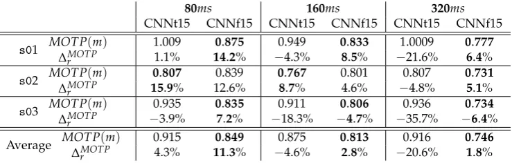
Table5 shows the comparison between these two options: training from scratch using s15 407

(columns CNNt15) and semi-synthetic training+fine tuning withs15 (columns CNNf15). The average 408

improvement of the latter approach varies between 1.8% and 11.3% with an average improvement 409

over all window lengths of 5.3%, while the training from scratch average improvement varies between 410

−20.6% and 4.3% with an average value of −7.0%. These differences show that the training+fine 411

tuning proposal outperforms training the network from scratch, thus validating our methodology. 412

Table 5. Results for the CNN proposal, either trained from scratch with sequences15 (columns CNNt15) or fine tuned with sequences15 (columns CNNf15).

80ms 160ms 320ms

CNNt15 CNNf15 CNNt15 CNNf15 CNNt15 CNNf15

s01 MOTP(m) ∆MOTP

r

1.009 0.875 0.949 0.833 1.0009 0.777 1.1% 14.2% −4.3% 8.5% −21.6% 6.4%

s02 MOTP_∆MOTP(m) r

0.807 0.839 0.767 0.801 0.807 0.731 15.9% 12.6% 8.7% 4.6% −4.8% 5.1%

s03 MOTP(m) ∆MOTP

r

0.935 0.835 0.911 0.806 0.936 0.734

−3.9% 7.2% −18.3% −4.7% −35.7% −6.4%

Average MOTP_∆MOTP(m) r

In spite of the relevant improvements with the fine tuning approach, they are still far from making 413

this suitable for further competitive exploitation in the ASL scenario (provided we have the GMBF 414

alternative), so that we next aim at increasing the amount of fine tuning material. 415

In our third experiment, we applied the fine tuning procedure using an additionalmoving speaker 416

sequence, that is, includings15 ands11 in the fine tuning subset. 417

Table6shows the results obtained by GMBF and CNN fine tuned withs15 ands11 (CNNf15+11 418

columns). In this case, we see additional improvements over using onlys15 for fine tuning, and there 419

is only one case in which CNNf15+11 does not outperforms SRP-PHAT (with a marginal degradation 420

of−0.3%). 421

Table 6. Relative improvements over SRP-PHAT for the strategy in [20] (columns GMBF); and the CNN fine tuned with sequencess15 ands11 (columns CNNf15+11)

80ms 160ms 320ms

GMBF CNNf15+11 GMBF CNNf15+11 GMBF CNNf15+11

s01 MOTP(m) ∆MOTP

r

0.795 0.805 0.686 0.750 0.588 0.706 22.1% 21.1% 24.6% 17.6% 29.1% 14.9%

s02 MOTP_∆MOTP(m) r

0.864 0.809 0.759 0.716 0.694 0.712

10.0% 15.7% 9.6% 14.8% 9.9% 7.5%

s03 MOTP(m) ∆MOTP

r

0.686 0.792 0.563 0.732 0.484 0.692 23.8% 12.0% 26.9% 4.9% 29.9% −0.3%

Average MOTP_∆MOTP(m) r

0.778 0.802 0.666 0.732 0.585 0.703 18.7% 16.2% 20.4% 12.4% 22.9% 7.5%

The CNN based approach shows again an average consistent improvement compared with 422

SRP-PHAT between 7.5% and 16.2%. 423

In this case, the newly added sequence (s11, with a duration of only 33 seconds) for fine tuning 424

corresponds to a randomly moving male speaker, and the results show that its addition contributes to 425

further improvements in the CNN based proposal, but it is still behind GMBF in all cases but two, but 426

with results getting closer. This suggests that a further increment in the fine tuning material should be 427

considered. 428

Our last experiment will consist of fine tuning the network including also additional static speaker 429

sequences. To assure that the training (including fine tuning) and testing material are fully independent, 430

we will fine tune withs15,s11 and with the static sequences that are not tested in each experiment 431

run, as shown in Table7. 432

Table 7.Fine tuning material used in the experiment corresponding to Table8columns CNNf15+11+st.

Test sequence Fine tuning sequences seq01 s15 +s11 +s02 +s03 seq02 s15 +s11 +s01 +s03 seq03 s15 +s11 +s01 +s02

Table8shows the results obtained for this fine tuning scenario, and the main conclusions are: 433

• The CNN based method exhibits much better average behavior than GMBF for all window sizes. 434

Average absolute improvement against SRP-PHAT for the CNN is more than 10 points higher 435

than for GMBF, reaching 31.3% in the CNN case and 20.7% for GMBF. 436

• Considering individual sequences, CNN is significantly better than GMBF for sequencess01 and 437

s02, and slightly worse fors03. 438

• Considering the best individual result, maximum improvement for the CNN is 41.6% (s01, 439

320ms), while the top result for GMBF is 29.9% (s03, 320ms). 440

• The effect of adding static sequences is beneficial, as expected, provided that the acoustic tuning 441

have varying heights and their position in the room is not strictly equal from sequence to 443

sequence. 444

• The improvements obtained are significant and come at the cost of additional fine tuning 445

sequences. However, this extra cost is still reasonable, as the extra fine tuning material is of 446

limited duration, around 400 seconds in average (6.65 minutes). 447

Table 8. Relative improvements over SRP-PHAT for the strategy in [20] (columns GMBF); and the CNN fine tuned with the sequences described in Table7(columns CNNf15+11+st)

80ms 160ms 320ms

GMBF CNNf15+11+st GMBF CNNf15+11+st GMBF CNNf15+11+st

s01 MOTP(m) ∆MOTP

r

0.795 0.607 0.686 0.540 0.588 0.485

22.1% 40.5% 24.6% 40.7% 29.1% 41.6%

s02 MOTP_∆MOTP(m) r

0.864 0.669 0.759 0.579 0.694 0.545

10.0% 30.3% 9.6% 31.1% 9.9% 29.2%

s03 MOTP(m) ∆MOTP

r

0.686 0.707 0.563 0.617 0.484 0.501

23.8% 21.4% 26.9% 19.9% 29.9% 27.4%

Average MOTP_∆MOTP(m) r

0.778 0.664 0.666 0.581 0.585 0.511

18.7% 30.6% 20.4% 30.6% 22.9% 32.8%

Finally, to summarize, Figure3shows the average MOTP relative improvements overSRP-PHAT 448

obtained by our CNN proposal using different fine tuning subsets, and its comparison with the GMBF 449

results, for all the signal window sizes. 450

Figure 3. MOTP relative improvements over SRP-PHAT for GMBF and CNN using different fine tuning subsets (for all window sizes).

From the results obtained by our proposal, it is clear that the highest contribution to the 451

improvements from the bare CNN training is the fine tuning procedure with limited data (CNNf15, 452

comparing Tables3and4), while the addition of additional fine tuning material consistently improves 453

the results (Tables6, and 8). It is again worth noticing that these improvements are consistently 454

independent of the gender of the considered speaker and whether there is a match or not between the 455

static or dynamic activity of the speakers being used in the fine tuning subsets. This suggest that the 456

network is actually learning the acoustic cues that are related to the localization problem, so that we 457

5. Conclusions 459

We have presented in this paper the first audio localization CNN that is trained end-to-end from 460

the audio signals to the source position. We show that this method is very promising, outperforming 461

the state-of-the-art methods [20,69] and those usingSRP-PHAT, given that sufficient fine tuning data is 462

available. In addition, our experiments show that the CNN method exhibits good resistance against 463

varying gender of the speaker and different window sizes compared with the baseline methods. Given 464

that the amount of data recordings for audio localization is limited at the moment, we have thus 465

proposed in the paper to first train the network using semi-synthetic data followed by fine tuning using 466

a small amount of real data. This has been a common strategy in other fields to prevent overfitting, 467

and we show in the paper that it significantly improves the system performance as compared with 468

training the network from scratch using real data. 469

In a future line of work we plan to improve the generation of semi-synthetic data including 470

reverberation effects and testing in detail the effects of gender and language in the system performance. 471

In addition we plan to include more real data by developing a large corpus for audio localization, 472

that will be made available to the scientific community for research purposes. Also, an extensive 473

evaluation will be carried out to asses the impact of the proposal with more complex acquisition 474

scenarios (comprising a higher number of microphone pairs). 475

Author Contributions: Conceptualization, Daniel Pizarro; Methodology, Writing - review & editing and 476

visualization, Daniel Pizarro, Juan Manuel Vera-Diaz and Javier Macias-Guarasa; Investigation, Juan Manuel 477

Vera-Diaz; Writing - original draft, Juan Manuel Vera-Diaz; Software, Daniel Pizarro and Juan Manuel Vera-Diaz; 478

Resources Javier Macias-Guarasa; Funding Acquisition, Daniel Pizarro and Javier Macias-Guarasa 479

Funding:Parts of this work were funded by the Spanish Ministry of Economy and Competitiveness under projects 480

HEIMDAL (TIN2016-75982-C2-1-R), ARTEMISA (TIN2016-80939-R), and SPACES-UAH (TIN2013-47630-C2-1-R), 481

and by the University of Alcalá under projects CCGP2017/EXP-025 and CCG2016/EXP-010. Juan 482

Manuel Vera-Diaz is funded by Comunidad de Madrid and FEDER under contract reference number 483

PEJD-2017-PRE/TIC-4626. 484

Conflicts of Interest:The authors declare no conflict of interest. 485

486

1. Torres-Solis, J.; Falk, T.H.; Chau, T. A review of indoor localization technologies: towards navigational 487

assistance for topographical disorientation. InAmbient Intelligence; InTech, 2010. 488

2. Ruiz-López, T.; Garrido, J.L.; Benghazi, K.; Chung, L. A survey on indoor positioning systems: foreseeing 489

a quality design. InDistributed Computing and Artificial Intelligence; Springer, 2010; pp. 373–380. 490

3. Mainetti, L.; Patrono, L.; Sergi, I. A survey on indoor positioning systems. Software, Telecommunications 491

and Computer Networks (SoftCOM), 2014 22nd International Conference on. IEEE, 2014, pp. 111–120. 492

4. Krizhevsky, A.; Sutskever, I.; Hinton, G.E. Imagenet classification with deep convolutional neural networks. 493

Advances in neural information processing systems, 2012, pp. 1097–1105. 494

5. Simonyan, K.; Zisserman, A. Very deep convolutional networks for large-scale image recognition. arXiv

495

preprint arXiv:1409.15562014. 496

6. DiBiase, J. A high-accuracy, low-latency technique for talker localization in reverberant environments 497

using microphone arrays. PhD thesis, Brown University, 2000. 498

7. Nunes, L.O.; Martins, W.A.; Lima, M.V.; Biscainho, L.W.; Costa, M.V.; Goncalves, F.M.; Said, A.; Lee, B. A 499

steered-response power algorithm employing hierarchical search for acoustic source localization using 500

microphone arrays.IEEE Transactions on Signal Processing2014,62, 5171–5183. 501

8. Cobos, M.; García-Pineda, M.; Arevalillo-Herráez, M. Steered response power localization of acoustic 502

passband signals. IEEE Signal Processing Letters2017,24, 717–721. 503

9. He, H.; Wang, X.; Zhou, Y.; Yang, T. A steered response power approach with trade-off prewhitening for 504

acoustic source localization.The Journal of the Acoustical Society of America2018,143, 1003–1007. 505

10. Salvati, D.; Drioli, C.; Foresti, G.L. Sensitivity-Based Region Selection in the Steered Response Power 506

11. Brandstein, M.S.; Silverman, H.F. A practical methodology for speech source localization with microphone 508

arrays.Computer Speech & Language1997,11, 91–126. doi:10.1006/csla.1996.0024. 509

12. DiBiase, J.; Silverman, H.; Brandstein, M. Robust localization in reverberant rooms. Microphone Arrays

510

2001, pp. 157–180. 511

13. Knapp, C.; Carter, G. The generalized correlation method for estimation of time delay.Acoustics, Speech

512

and Signal Processing, IEEE Transactions on1976,24, 320 – 327. doi:10.1109/TASSP.1976.1162830. 513

14. Zhang, C.; Florencio, D.; Zhang, Z. Why does PHAT work well in low noise, reverberative environments? 514

Acoustics, Speech and Signal Processing, 2008. ICASSP 2008. IEEE International Conference on, 2008, pp. 515

2565 –2568. doi:10.1109/ICASSP.2008.4518172. 516

15. Dmochowski, J.P.; Benesty, J. Steered Beamforming Approaches for Acoustic Source Localization. InSpeech

517

Processing in Modern Communication; Cohen, I.; Benesty, J.; Gannot, S., Eds.; Springer Berlin Heidelberg, 518

2010; Vol. 3,Springer Topics in Signal Processing, pp. 307–337. 10.1007/978-3-642-11130-3_12. 519

16. Cobos, M.; Marti, A.; Lopez, J. A modified SRP-PHAT functional for robust real-time sound source 520

localization with scalable spatial sampling.Signal Processing Letters, IEEE2011,18, 71–74. 521

17. Butko, T.; Gonzalez Pla, F.; Segura Perales, C.; Nadeu Camprubí, C.; Hernando Pericás, F.J. Two-source 522

acoustic event detection and localization: online implementation in a smart-room. Proceedings of the 17th 523

European Signal Processing Conference (EUSIPCO’11), 2011, pp. 1317–1321. 524

18. Habets, E.A.P.; Benesty, J.; Gannot, S.; Cohen, I. The MVDR Beamformer for Speech Enhancement. InSpeech

525

Processing in Modern Communication; Cohen, I.; Benesty, J.; Gannot, S., Eds.; Springer Berlin Heidelberg, 526

2010; Vol. 3,Springer Topics in Signal Processing, pp. 225–254. 10.1007/978-3-642-11130-3_9. 527

19. Marti, A.; Cobos, M.; Lopez, J.J.; Escolano, J. A steered response power iterative method for high-accuracy 528

acoustic source localization. The Journal of the Acoustical Society of America 2013, 134, 2627–2630, 529

[https://doi.org/10.1121/1.4820885]. doi:10.1121/1.4820885. 530

20. Velasco, J.; Pizarro, D.; Macias-Guarasa, J. Source Localization with Acoustic Sensor Arrays 531

Using Generative Model Based Fitting with Sparse Constraints. Sensors 2012, 12, 13781–13812. 532

doi:10.3390/s121013781. 533

21. Padois, T.; Sgard, F.; Doutres, O.; Berry, A. Comparison of acoustic source localization methods in time 534

domain using sparsity constraints. 2015. cited By 0. 535

22. Velasco, J.; Pizarro, D.; Macias-Guarasa, J.; Asaei, A. TDOA Matrices: Algebraic Properties and Their 536

Application to Robust Denoising With Missing Data. IEEE Transactions on Signal Processing 2016, 537

64, 5242–5254. doi:10.1109/TSP.2016.2593690. 538

23. Compagnoni, M.; Pini, A.; Canclini, A.; Bestagini, P.; Antonacci, F.; Tubaro, S.; Sarti, A. A 539

Geometrical-Statistical Approach to Outlier Removal for TDOA Measurements. IEEE Transactions on Signal

540

Processing2017,65, 3960–3975. doi:10.1109/TSP.2017.2701311. 541

24. Salari, S.; Chan, F.; Chan, Y.T.; Read, W. TDOA Estimation With Compressive Sensing Measurements 542

and Hadamard Matrix. IEEE Transactions on Aerospace and Electronic Systems 2018, pp. 1–1. 543

doi:10.1109/TAES.2018.2826230. 544

25. Murray, J.C.; Erwin, H.R.; Wermter, S. Robotic sound-source localisation architecture using cross-correlation 545

and recurrent neural networks. Neural Networks2009,22, 173 – 189. What it Means to Communicate, 546

doi:https://doi.org/10.1016/j.neunet.2009.01.013. 547

26. Deleforge, A. Acoustic Space Mapping: A Machine Learning Approach to Sound Source Separation and 548

Localization. Theses, Université de Grenoble, 2013. 549

27. Salvati, D.; Drioli, C.; Foresti, G.L. On the use of machine learning in microphone array beamforming 550

for far-field sound source localization. 2016 IEEE 26th International Workshop on Machine Learning for 551

Signal Processing (MLSP), 2016, pp. 1–6. doi:10.1109/MLSP.2016.7738899. 552

28. Rascon, C.; Meza, I. Localization of sound sources in robotics: A review. Robotics and Autonomous Systems

553

2017,96, 184 – 210. doi:https://doi.org/10.1016/j.robot.2017.07.011. 554

29. Stoica, P.; Li, J. Lecture Notes - Source Localization from Range-Difference Measurements. IEEE Signal

555

Processing Magazine2006,23, 63–66. doi:10.1109/SP-M.2006.248717. 556

30. Cobos, M.; García-Pineda, M.; Arevalillo-Herráez, M. Steered Response Power Localization of Acoustic 557

Passband Signals.IEEE Signal Processing Letters2017,24, 717–721. doi:10.1109/LSP.2017.2690306. 558

31. Omologo, M.; Svaizer, P. Use Of The Cross-Power-Spectrum Phase In Acoustic Event Location. IEEE Trans.

559

32. Dmochowski, J.; Benesty, J.; Affes, S. A Generalized Steered Response Power Method for Computationally 561

Viable Source Localization.Audio, Speech, and Language Processing, IEEE Transactions on2007,15, 2510 –2526. 562

doi:10.1109/TASL.2007.906694. 563

33. Badali, A.; Valin, J.M.; Michaud, F.; Aarabi, P. Evaluating real-time audio localization algorithms for 564

artificial audition in robotics. Intelligent Robots and Systems, 2009. IROS 2009. IEEE/RSJ International 565

Conference on, 2009, pp. 2033 –2038. doi:10.1109/IROS.2009.5354308. 566

34. Do, H.; Silverman, H. SRP-PHAT methods of locating simultaneous multiple talkers using a frame of 567

microphone array data. Acoustics Speech and Signal Processing (ICASSP), 2010 IEEE International 568

Conference on, 2010, pp. 125 –128. doi:10.1109/ICASSP.2010.5496133. 569

35. Schmidt, R. Multiple emitter location and signal parameter estimation. Antennas and Propagation, IEEE

570

Transactions on1986,34, 276 – 280. doi:10.1109/TAP.1986.1143830. 571

36. Goodfellow, I.; Bengio, Y.; Courville, A.; Bengio, Y.Deep learning; Vol. 1, MIT press Cambridge, 2016. 572

37. Krizhevsky, A.; Sutskever, I.; Hinton, G.E. Imagenet classification with deep convolutional neural networks. 573

Advances in neural information processing systems, 2012, pp. 1097–1105. 574

38. He, K.; Zhang, X.; Ren, S.; Sun, J. Deep Residual Learning for Image Recognition. 2016 IEEE Conference on

575

Computer Vision and Pattern Recognition (CVPR)2016, pp. 770–778. 576

39. Hinton, G.; Deng, L.; Yu, D.; Dahl, G.E.; Mohamed, A.r.; Jaitly, N.; Senior, A.; Vanhoucke, V.; Nguyen, P.; 577

Sainath, T.N.; others. Deep neural networks for acoustic modeling in speech recognition: The shared views 578

of four research groups.IEEE Signal processing magazine2012,29, 82–97. 579

40. Graves, A.; Jaitly, N. Towards end-to-end speech recognition with recurrent neural networks. International 580

Conference on Machine Learning, 2014, pp. 1764–1772. 581

41. Deng, L.; Platt, J.C. Ensemble deep learning for speech recognition. INTERSPEECH, 2014. 582

42. Steinberg, B.Z.; Beran, M.J.; Chin, S.H.; Howard, J.H. A neural network approach to source localization. 583

The Journal of the Acoustical Society of America1991,90, 2081–2090,[https://doi.org/10.1121/1.401635]. 584

doi:10.1121/1.401635. 585

43. Datum, M.S.; Palmieri, F.; Moiseff, A. An artificial neural network for sound localization using binaural 586

cues. The Journal of the Acoustical Society of America1996,100, 372–383,[https://doi.org/10.1121/1.415854]. 587

doi:10.1121/1.415854. 588

44. Youssef, K.; Argentieri, S.; Zarader, J.L. A learning-based approach to robust binaural sound localization. 589

2013 IEEE/RSJ International Conference on Intelligent Robots and Systems, 2013, pp. 2927–2932. 590

doi:10.1109/IROS.2013.6696771. 591

45. Xiao, X.; Zhao, S.; Zhong, X.; Jones, D.L.; Siong, C.E.; Li, H. A learning-based approach to direction of 592

arrival estimation in noisy and reverberant environments. 2015 IEEE International Conference on Acoustics,

593

Speech and Signal Processing (ICASSP)2015, pp. 2814–2818. 594

46. Ma, N.; Brown, G.; May, T., Exploiting deep neural networks and head movements for binaural localisation 595

of multiple speakers in reverberant conditions. InProceedings of Interspeech 2015; ISCA, 2015; pp. 3302–3306. 596

47. Takeda, R.; Komatani, K. Discriminative multiple sound source localization based on deep neural networks 597

using independent location model.2016 IEEE Spoken Language Technology Workshop (SLT)2016, pp. 603–609. 598

48. Takeda, R.; Komatani, K. Sound source localization based on deep neural networks with directional 599

activate function exploiting phase information. 2016 IEEE International Conference on Acoustics, Speech and

600

Signal Processing (ICASSP)2016, pp. 405–409. 601

49. Takeda, R.; Komatani, K. Unsupervised adaptation of deep neural networks for sound source localization 602

using entropy minimization. 2017 IEEE International Conference on Acoustics, Speech and Signal 603

Processing (ICASSP), 2017, pp. 2217–2221. doi:10.1109/ICASSP.2017.7952550. 604

50. Sun, Y.; Chen, J.; Yuen, C.; Rahardja, S. Indoor Sound Source Localization With Probabilistic Neural 605

Network.IEEE Transactions on Industrial Electronics2018,65, 6403–6413. doi:10.1109/TIE.2017.2786219. 606

51. Chakrabarty, S.; Habets, E.A.P. Multi-Speaker Localization using Convolutional Neural Network Trained 607

with Noise. ML4Audio Workshop at NIPS, 2017. 608

52. Yalta, N.; Nakadai, K.; Ogata, T. Sound source localization using deep learning models. Journal of Robotics

609

and Mechatronics2017,29, 37–48. doi:10.20965/jrm.2017.p0037. 610

53. Ferguson, E.L.; Williams, S.B.; Jin, C.T. Sound Source Localization in a Multipath Environment Using 611

54. Hirvonen, T. Classification of Spatial Audio Location and Content Using Convolutional Neural Networks. 613

138th Audio Engineering Society Convention 2015, 2015, Vol. 2. 614

55. He, W.; Motlícek, P.; Odobez, J. Deep Neural Networks for Multiple Speaker Detection and Localization. 615

CoRR2017,abs/1711.11565,[1711.11565]. 616

56. Salvati, D.; Drioli, C.; Foresti, G.L. Exploiting CNNs for Improving Acoustic Source Localization in 617

Noisy and Reverberant Conditions. IEEE Transactions on Emerging Topics in Computational Intelligence2018, 618

2, 103–116. doi:10.1109/TETCI.2017.2775237. 619

57. Ma, W.; Liu, X. Phased Microphone Array for Sound Source Localization with Deep Learning. CoRR2018, 620

abs/1802.04479,[1802.04479]. 621

58. Thuillier, E.; Gamper, H.; Tashev, I. Spatial audio feature discovery with convolutional neural networks. 622

Proc. IEEE International Conference on Acoustics, Speech and Signal Processing (ICASSP). IEEE, 2018. 623

59. Pertilä, P.; Cakir, E. Robust direction estimation with convolutional neural networks based steered response 624

power. 2017 IEEE International Conference on Acoustics, Speech and Signal Processing (ICASSP), 2017, pp. 625

6125–6129. doi:10.1109/ICASSP.2017.7953333. 626

60. Le, Q.V.; Ngiam, J.; Coates, A.; Lahiri, A.; Prochnow, B.; Ng, A.Y. On optimization methods for deep 627

learning. Proceedings of the 28th International Conference on International Conference on Machine 628

Learning. Omnipress, 2011, pp. 265–272. 629

61. Allen, J.B.; Berkley, D.A. Image method for efficiently simulating small-room acoustics. The Journal of the

630

Acoustical Society of America1979,65, 943–950,[https://doi.org/10.1121/1.382599]. doi:10.1121/1.382599. 631

62. Velasco, J.; Martín-Arguedas, C.J.; Macias-Guarasa, J.; Pizarro, D.; Mazo, M. Proposal and validation of an 632

analytical generative model of SRP-PHAT power maps in reverberant scenarios.Signal Processing2016, 633

119, 209 – 228. doi:http://dx.doi.org/10.1016/j.sigpro.2015.08.003. 634

63. Lathoud, G.; Odobez, J.M.; Gatica-Perez, D. AV16.3: An Audio-Visual Corpus for Speaker Localization 635

and Tracking. Procceedings of the MLMI; Bengio, S.; Bourlard, H., Eds. Springer-Verlag, 2004, Vol. 3361, 636

Lecture Notes in Computer Science, pp. 182–195. 637

64. Moore, D.C. The IDIAP Smart Meeting Room. Technical report, IDIAP Research Institute, Switzerland, 638

2004. 639

65. Lathoud, G. AV16.3 Dataset.http://www.idiap.ch/dataset/av16-3/(accessed on 11 october 2012), 2004. 640

66. Association, E.E.L.R. Albayzin corpus. http://catalogue.elra.info/en-us/repository/browse/albayzin-641

corpus/b50c9628a9dd11e7a093ac9e1701ca0253c876277d534e7ca4aca155a5611535/. 642

67. Moreno, A.; Poch, D.; Bonafonte, A.; Lleida, E.; Llisterri, J.; Mariño, J.B.; Nadeu, C. Albayzin speech 643

database: design of the phonetic corpus. EUROSPEECH. ISCA, 1993. 644

68. Kingma, D.P.; Ba, J. Adam: A method for stochastic optimization.arXiv preprint arXiv:1412.69802014. 645

69. Velasco-Cerpa, J.F. Mathematical Modelling and Optimization Strategies for Acoustic Source Localization 646

in Reverberant Environments. PhD thesis, Escuela Politécnica Superior. University of Alcalá (Spain), 2017. 647

70. Mostefa, D.; Garcia, M.; Bernardin, K.; Stiefelhagen, R.; McDonough, J.; Voit, M.; Omologo, M.; Marques, 648

F.; Ekenel, H.; Pnevmatikakis, A. Clear evaluation plan, document CHIL-CLEAR-V1.1 2006-02-21.http: 649

//www.clear-evaluation.org/clear06/downloads/chil-clear-v1.1-2006-02-21.pdf(accessed on 11 october 650