The Relevance of Inter-regional Trade Data
Produced by the 2012 Commodity Flow Survey
for Multi-regional CGE Modelling
CoPS Working Paper No. G-275, August 2017
The Centre of Policy Studies (CoPS), incorporating the IMPACT project, is a research centre at Victoria University devoted to quantitative analysis of issues relevant to economic policy. Address: Centre of Policy Studies, Victoria University, PO Box 14428, Melbourne, Victoria, 8001 home page: www.vu.edu.au/CoPS/ email: [email protected] Telephone +61 3 9919 1877
Glyn Wittwer
Centre of Policy Studies, Victoria University
The relevance of inter-regional trade data produced by the 2012 Commodity Flow Survey for multi-regional CGE modelling
Glyn Wittwer, Centre of Policy Studies, August 2017
Abstract
The objective of this study is to assess the suitability of Commodity Flow Survey (CFS) data released by the US Census Bureau as a check on the estimates of inter-regional trade generated in creating the USAGE-TERM master database.
A close inspection of the Census Bureau’s CFS data indicate that they record movements to and from transport nodes. In some cases, transport nodes may align with production origins and final use destinations. In other cases, nodes appear to be intermediate points rather than origins or final destinations. This implies that CFS data are often incompatible with the trade flows in a CGE database.
Merchandise, that is primary and manufacturing commodities, account for no more than 15% of GDP in the U.S. economy. Therefore, even comprehensive merchandise trade flow data would have limited use in a CGE database. The usefulness of the CFS data is diminished further by its concentration on bulky goods, which account for a small fraction of total trade flows. Bulky trade flows may account for a substantial proportion of the volume of trade but make a small contribution to total economic activity. Mining products excluding oil and gas account for 50.9% of the recorded weight in the survey, but just 3.9% of the value of trades – and only 0.3% of GDP. The CFS data might be useful for examining transport logistics but are of little use in CGE database preparation.
There is no evidence that the CFS data supersedes the Horridge gravity method of allocating inter-regional trades. However, CFS data point to the desirability of noting the difference between transport in the Mississippi basin and elsewhere. The basin relies heavily on water transport for moving agricultural, mining and fuel products.
JEL classification: R11, R13, R15, C68
Contents
1. Introduction 1
2. The sectoral classification 4 3. What are the Census Bureau data recording? 12 4. What can multi-regional CGE modellers learn from the bureau’s sample data? 16
5. Concluding remarks 17
References 17
Figures
Figure 1: Origin shares of cereal grains destined for Missouri in survey data and the USAGE-TERM
TRADE matrix 14
Figure 2: Origin shares of cereal grains destined for Louisiana in survey data and the USAGE-TERM
TRADE matrix 15
Figure 3: Destination shares of alcohol originating in California in survey data and the
USAGE-TERM TRADE matrix 16
Tables
Table 1: Top 5 SCTG commodities in shipments by each NAICS industry 6
1. Introduction
1.1 The TERM methodology
Mark Horridge introduced the TERM (The Enormous Regional Model) methodology to advance significantly the modeling detail in sub-national multi-regional CGE models (Horridge et al., 2005). Until his contribution, there had been a tendency for sub-national regions to contain fewer sectors than the published national table. However, data are
available from a number of sources to provide regional detail that is more disaggregated than a published national table.
Agricultural bureaus such as the USDA provide statistics that are available at a regional level in more detail than are provided in the national input-output table. Indeed, with a sufficient level of disaggregation, a clear picture emerges as to which crops are grown where. For example, tropical fruits are confined mostly to tropical regions. In the context of agriculture, splitting of the database into small regions enables us to make use of additional small region data to improve the depiction of resource management. For example, Wittwer (2017) used available data from the USDA to devise water accounts so as to examine the impact of drought on agriculture in California. This followed Dixon et al. (2011) who made extensive modifications to the database and theory to depict agriculture in Australia’s Murray-Darling Basin in a bottom-up, multi-regional CGE model.
Highly disaggregated data at the regional level enhance our depiction of differences between regions. For example, if we split health sectors into as many sectors as are supported by available employment data from the census, then we might see the extent of disparities between regions concerning specialist health services.
Statistics are also available for mining and energy outputs at the regional level. In the case of manufacturing and service sectors, which tend to be relatively labor-intensive, employment data are available from a nation’s census at a finely disaggregated level in both the sectoral and regional dimensions (Wittwer and Horridge, 2009).
Regional electricity generation data by fuel type assist in splitting generation into several sectors. Splitting electricity in different sectors is an important step in bringing greenhouse gas accounts into a CGE model (Adams and Parmenter, 2013).
A major motivation for representing more sectors than are available in the national input-output table is that when the national sectors are split into regions, the TERM methodology assumes that a given industry has identical cost structures in each region. This is more defensible for a specific crop such as pineapples or almonds than it is for a broad sector such as crops. An obvious example is electricity generation. Coal-generated electricity has
dominated generation in West Virginia but contributes less than 1% to electricity generation within California. By splitting national electricity generation by fuel type, we can use
estimates of regional shares of each type of generation to reflect the difference in composition of electricity generation in each region.
In many nations, international trade are available by port. These data are compiled from customs entries and for merchandise are relatively comprehensive. The TERM methodology assigns exports by port rather than origin in the USE matrix (which includes the commodity, user and destination but not the regional origin), and details the origin and destination (port) in the domestic part of the inter-regional TRADE matrix (which excludes the user). Similarly, international imports are assigned to the port of import in the USE matrix, while the port origin and user destination are assigned in the import part of the inter-regional TRADE matrix. For merchandise, the international port is based on actual data.
Horridge devised a gravity formula to distribute supplies from each regional origin so as to satisfy regional demands. In many cases, the gravity formula does little. For example, since California accounts for virtually all of US almond production, and since imports of almonds are negligible, the origin of almonds used in each destination is known. That is, in this case the gravity assumption does almost nothing.
Clearly, there is always room for improvement in devising a multi-regional database using the TERM methodology. Better data may become available, for example, on disaggregated household consumption expenditure by region. As noted by Horridge (2012), the processing of a TERM master database is highly automated, so that improved information can be added to the multi-regional CGE database with relative ease.
1.2 Evaluating the usefulness of CFS data
International trade data are available at least for merchandise commodities in a global model, and play an important part in the database of the global CGE GTAP model. However, a substantial proportion of most economies consists of services and utilities, which together account for a large share of GDP while being relatively less traded than merchandise.
Tourism and education are exceptions among services, with growing international trade. The most important data required in either a global model or sub-national multi-regional model are estimates of regional production and consumption.
The remainder of this study examines the Commodity Flow Survey (CFS) data prepared by the US Census Bureau. Can these data play a role in improving the database of a sub-national multi-regional CGE model?
2. The sectoral classification
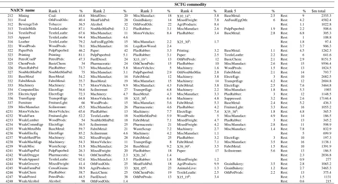
In searching for commodity details, we must note the following from the CFS users’ guide: the NAICS field is defined as the Industry classification of shipper (Appendix A of guide). It does not refer to the commodity. Rather, the Standard Classification of Transported Goods (SCTG) field is the 2-digit SCTG commodity code of the shipment.
An inspection of the 45 NAICS categories shows that 17 are wholesale trade sectors. The NAICS category shows the industry that has taken responsibility for the shipping. Table 1 shows the main SCTG commodities for which each NAICS industry takes responsibility for shipping in the data sample.
In some instances, there is a close correspondence between NAICS and SCTG. In others, this is not the case.
For example, 98% of the shipments of the wholesale alcohol sector (NAICS 4248) are of alcohol. But 18% of the NAICS sector mining’s (NAICS 212) shipments are of
One interpretation of the spread of 2-digit SCTG commodities shipped by many industries is that the NAICS sector responsible for shipment may move one type of commodity in one direction, and move an entirely different commodity on the return journey.
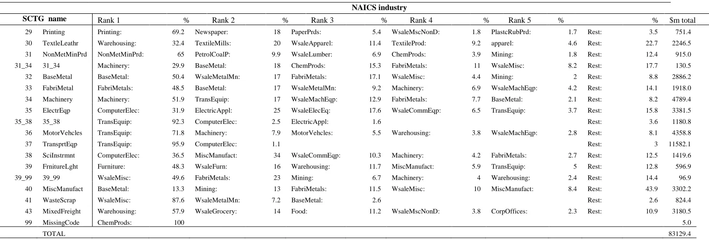
Table 2 shows shares of each SCTG commodity shipped by various NAICS industries. SCTG code 00 covers data for which the commodity group is suppressed. Around 94% of the value of these data is shipped by NAICS industry 336 (transport equipment).
Table 2 shows that SCTG commodity 05 (meat and fish products) is shipped mainly by the food industry (NAICS 311, 85.6%) with wholesale groceries (NAICS 4244, 13%) and warehousing (NAICS 4931, 1.5%) being responsible for smaller shares.
Table 1. Top 5 SCTG commodities in shipments by each NAICS industry: % shares in shipments
SCTG commodity
NAICS name Rank 1 % Rank 2 % Rank 3 % Rank 4 % Rank 5 % % $m total
212 Mining Coal: 44.6 MetalOres: 20 MiscManufact: 18 X10_14a: 5.8 BaseMetal: 2.5 Rest: 9 2355.3
311 Food OthFoodOils: 40.4 MeatFishPrd: 28 GrainBakery: 14 MixedFreight: 7.8 AnFeedEggOth: 6 Rest: 4.2 4582.4
312 BeverageTob Tobacco: 36.5 Alcohol: 32 OthFoodOils: 22 AgriProducts: 8.4 Rest: 1.1 1022.8
313 TextileMills TextleLeathr: 87.1 NonMetMinPrd: 3.2 PlasRubber: 3.1 MiscManufact: 2.6 PulpPaperbrd: 1.9 Rest: 2.2 508.6 314 TextileProd TextleLeathr: 67.6 MiscManufact: 11 MotorVehcles: 8.4 PlasRubber: 3.4 BaseMetal: 2.8 Rest: 6.8 305.3
315 Apparel TextleLeathr: 94.4 MiscManufact: 4.6 Rest: 1 108.8
316 Leather TextleLeathr: 79.2 AnFeedEggOth: 15 MiscManufact: 2.2 X25_30b: 1.7 Rest: 1.8 97.4
321 WoodProds WoodProds: 78.1 MiscManufact: 16 LogsRawWood: 2.4 Rest: 3.7 906.3
322 PaperPrds PulpPaperbrd: 46.2 Paper: 42 PlasRubber: 3.3 Printing: 3.2 BaseMetal: 1.1 Rest: 4.5 1262.3 323 Printing Printing: 81.1 PulpPaperbrd: 5.1 PlasRubber: 3.1 Paper: 2.5 TextleLeathr: 2.2 Rest: 6 641.6 324 PetrolCoalP PetrolPrds: 47.3 FuelDiesel: 24 X15_19 c: 13 OthPetProds: 12 BasicChem: 2.1 Rest: 2.9 8151.5 325 ChemProds BasicChem: 34 Pharmaceutic: 24 OthChemPrds: 15 PlasRubber: 10 MiscManufact: 2.6 Rest: 15 9596.4 326 PlastcRubPrd PlasRubber: 73.7 MiscManufact: 5.8 MotorVehcles: 5 Machinery: 1.6 WoodProds: 1.5 Rest: 13 1824.5 327 NonMetMinPrd NonMetMinPrd: 75 MiscManufact: 3.1 PulpPaperbrd: 2.9 OthNonMetMin: 2.8 FabriMetal: 2.1 Rest: 14 793.7 331 BaseMetal BaseMetal: 54.2 MiscManufact: 16 FabriMetal: 12 Machinery: 3.8 ElectrEqp: 3 Rest: 10 2682.5 332 FabriMetals FabriMetal: 35.7 BaseMetal: 19 MiscManufact: 15 Machinery: 14 TransprtEqp: 4.2 Rest: 12 2604.8 333 Machinery Machinery: 71.7 MotorVehcles: 9.9 MiscManufact: 4.3 FabriMetal: 3.8 ElectrEqp: 2.5 Rest: 7.6 3464.8 334 ComputerElec ElectrEqp: 56.6 SciInstrmnt: 27 TransprtEqp: 6.8 Machinery: 2.2 MiscManufact: 1.8 Rest: 5.3 1903 335 ElectricAppl ElectrEqp: 72.3 Machinery: 4.7 BaseMetal: 4.3 MiscManufact: 3.3 PlasRubber: 3 Rest: 12 1148.5 336 TransEquip TransprtEqp: 64.8 MotorVehcles: 18 X35_38d: 6.4 Machinery: 4.8 Suppressed: 3.2 Rest: 2.6 17146.4 337 Furniture FrnitureLght: 66 WoodProds: 15 MiscManufact: 5.6 FabriMetal: 5.3 BaseMetal: 2.4 Rest: 5.2 436.3 339 MiscManufact SciInstrmnt: 45.5 MiscManufact: 26 Pharmaceutic: 4.6 PlasRubber: 4.2 FrnitureLght: 3.3 Rest: 16 1055.2 4231 MotorVehcles MotorVehcles: 65.6 PlasRubber: 13 Machinery: 7.7 ElectrEqp: 7.4 X35_38d: 1.8 Rest: 4.8 365.5 4232 WsaleFurn FrnitureLght: 52.2 TextleLeathr: 18 NonMetMinPrd: 5.9 WoodProds: 5 MiscManufact: 4.9 Rest: 14 186.5 4233 WsaleLumber WoodProds: 54 NonMetMinPrd: 18 FabriMetal: 7.1 MixedFreight: 4.7 PlasRubber: 3 Rest: 13 345.2 4234 WsaleCommEqp ElectrEqp: 36.5 SciInstrmnt: 25 Pharmaceutic: 21 MixedFreight: 4.2 MiscManufact: 2.8 Rest: 11 598.9 4235 WsaleMetalMn BaseMetal: 59.7 FabriMetal: 21 WasteScrap: 7.2 Machinery: 2.7 MiscManufact: 1.4 Rest: 7.8 832.9
4236 WsaleElecEq ElectrEqp: 85.2 SciInstrmnt: 4.6 Machinery: 4.2 MiscManufact: 1.1 Rest: 5 699.9
4237 WsaleHardPlm Machinery: 30.2 MixedFreight: 28 FabriMetal: 25 PlasRubber: 3.2 ElectrEqp: 3 Rest: 10 197.3 4238 WsaleMachEqp Machinery: 54.3 MotorVehcles: 11 TransprtEqp: 8 FabriMetal: 7.1 MiscManufact: 3.5 Rest: 16 1138.1 4239 WsaleMisc WasteScrap: 51.9 MiscManufact: 24 BaseMetal: 9.2 X39_99e: 3.5 FabriMetal: 1.5 Rest: 10 1391.9 4241 WsalePaprPrd PulpPaperbrd: 26.3 MixedFreight: 20 PlasRubber: 18 Paper: 17 SciInstrmnt: 5.6 Rest: 13 186.5
4242 WsaleDruggst Pharmaceutic: 94.1 OthChemPrds: 2.3 X20_24f: 1.4 Rest: 2.3 2036.8
4243 WsaleApparel TextleLeathr: 92.6 MiscManufact: 3.5 PlasRubber: 1.8 MixedFreight: 1.2 Rest: 0.9 277
4244 WsaleGrocery MixedFreight: 41.4 OthFoodOils: 25 MeatFishPrd: 18 AgriProducts: 9.9 GrainBakery: 3.5 Rest: 2.8 1065.2 4245 WsaleFarmPrd CerealGrains: 38.9 AgriProducts: 33 X01_05g: 23 AnimalsLive: 1.3 GrainBakery: 1.2 Rest: 2.7 3465.3 4246 WsaleChem PlasRubber: 38.7 BasicChem: 25 OthChemPrds: 19 TextleLeathr: 2.5 OthPetProds: 2.2 Rest: 13 375.4
4247 WsalePetrol PetrolPrds: 44.5 FuelDiesel: 38 OthPetProds: 13 X15_19h: 3.4 Rest: 1.5 1131
4248 WsaleAlcohol Alcohol: 98 OthFoodOils: 1.4 Rest: 0.6 215
Table 1 (cont.). Top 5 SCTG commodities in shipments by each NAICS industry: % shares in shipments
SCTG commodity
NAICS name Rank 1 % Rank 2 % Rank 3 % Rank 4 % Rank 5 % % $m total
4249 WsaleMscNonD MixedFreight: 18.4 Tobacco: 13 Fertilizers: 12 AgriProducts: 11 OthChemPrds: 10 Rest: 36 661 4541 ElecOrderH TextleLeathr: 34.3 MiscManufact: 32 OthChemPrds: 12 Pharmaceutic: 11 ElectrEqp: 3.7 Rest: 7.3 163.5
45431 DirectSell FuelDiesel: 46.8 OthPetProds: 42 PetrolPrds: 9.5 Rest: 1.4 79.2
4931 Warehousing MixedFreight: 47.9 TextleLeathr: 19 MiscManufact: 4.6 MotorVehcles: 4.3 Pharmaceutic: 2.9 Rest: 21 3841.5
5111 Newspaper Printing: 89.9 Paper: 6.2 X25_30a: 2.8 Rest: 1.1 154.2
551114 CorpOffices OthPetProds: 40.2 Pharmaceutic: 8.7 OthChemPrds: 7.3 TextleLeathr: 7 MixedFreight: 6.6 Rest: 30 1123.2
TOTAL 83129.4
a Composite of commodity 25 to 30.
Table 2. Top 5 NAICS industries responsible for the shipping of each SCTG commodity: % shares
NAICS industry
SCTG name Rank 1 % Rank 2 % Rank 3 % Rank 4 % Rank 5 % % $m total
00 Suppressed TransEquip: 93.7 ChemProds: 1.8 Rest: 4.4 576.9
01 AnimalsLive WsaleFarmPrd: 97.3 WsaleMscNonD: 1.8 Rest: 1 45.7
01_05 Composite agri WsaleFarmPrd: 94.4 Warehousing: 1.8 Food: 1.6 Rest: 2.2 853.9
02 CerealGrains WsaleFarmPrd: 94.8 WsaleMscNonD: 3 Warehousing: 1.2 Rest: 0.9 1421.9
03 AgriProducts WsaleFarmPrd: 75.4 WsaleGrocery: 7 BeverageTob: 5.8 Food: 5.2 WsaleMscNonD: 4.9 Rest: 1.7 1500.8
04 AnFeedEggOth Food: 54.1 ChemProds: 14 WsaleMscNonD: 10 Warehousing: 8.7 WsaleFarmPrd: 6.8 Rest: 6.7 510.3
05 MeatFishPrd Food: 85.6 WsaleGrocery: 13 Warehousing: 1.5 Rest: 0.1 1471.4
06 GrainBakery Food: 85.8 WsaleFarmPrd: 5.5 WsaleGrocery: 5 Warehousing: 2.2 Rest: 1.5 753.8
06_09 Composite food Food: 70 ChemProds: 11 WsaleFarmPrd: 10.5 BeverageTob: 5.3 Rest: 3.2 91.5
07 OthFoodOils Food: 70.7 WsaleGrocery: 10 BeverageTob: 8.6 ChemProds: 4.3 Warehousing: 3.8 Rest: 2.6 2617.6
08 Alcohol BeverageTob: 56.1 WsaleAlcohol: 36 ChemProds: 4.8 CorpOffices: 1 Rest: 2.1 584.4
09 Tobacco BeverageTob: 78.9 WsaleMscNonD: 18 Warehousing: 2.5 Rest: 1 472.5
10 BuildStone NonMetMinPrd: 52.7 Mining: 28 WsaleLumber: 14.7 WsaleFurn: 1.9 CorpOffices: 1.3 Rest: 1.5 17.5
10_14 Comp. non-metl Mining: 80.4 BaseMetal: 7.7 ChemProds: 5.6 NonMetMinPrd: 2.5 Rest: 3.7 168.5
11 Sands Mining: 63.8 NonMetMinPrd: 19 ChemProds: 13.2 Rest: 4.1 43.2
12 GravelStone Mining: 75.7 ChemProds: 7.7 NonMetMinPrd: 6 WsaleLumber: 4.5 PetrolCoalP: 3.3 Rest: 2.7 49.3
13 OthNonMetMin Mining: 50.8 NonMetMinPrd: 20 ChemProds: 18.6 Warehousing: 2.5 WsaleMachEqp: 1.7 Rest: 6.2 111.0
14 MetalOres Mining: 78.2 BaseMetal: 11 ChemProds: 5.5 CorpOffices: 2.2 WsaleMetalMn: 1.4 Rest: 2.1 610.7
15 Coal Mining: 99.1 Rest: 0.9 1059.4
15_19 Comp. energy PetrolCoalP: 86.4 ChemProds: 4.5 CorpOffices: 3.6 WsalePetrol: 3.3 Mining: 1.9 Rest: 0.3 1182.0
17 PetrolPrds PetrolCoalP: 83 WsalePetrol: 11 ChemProds: 4.3 Warehousing: 1.1 Rest: 0.8 4647.0
18 FuelDiesel PetrolCoalP: 78.3 WsalePetrol: 18 DirectSell: 1.5 CorpOffices: 1.2 ChemProds: 1 Rest: 0.4 2444.3 19 OthPetProds PetrolCoalP: 50.5 CorpOffices: 24 ChemProds: 11 WsalePetrol: 7.6 Warehousing: 2.9 Rest: 4.1 1880.9
20 BasicChem ChemProds: 87.6 PetrolCoalP: 4.6 WsaleChem: 2.5 Warehousing: 1.1 Rest: 4.1 3724.9
20_24 Comp. chemicals ChemProds: 64 PetrolCoalP: 12 WsaleDruggst: 8.8 BaseMetal: 3.4 Warehousing: 3 Rest: 9.2 319.1 21 Pharmaceutic ChemProds: 49.5 WsaleDruggst: 41 WsaleCommEqp: 2.7 Warehousing: 2.4 CorpOffices: 2.1 Rest: 1.9 4630.7 22 Fertilizers ChemProds: 54.6 WsaleMscNonD: 24 Warehousing: 8.9 Mining: 7.2 WsaleFarmPrd: 2.7 Rest: 3.2 335.9 23 OthChemPrds ChemProds: 72.5 CorpOffices: 4.2 PetrolCoalP: 3.8 WsaleChem: 3.6 WsaleMscNonD: 3.5 Rest: 12.3 1923.5 24 PlasRubber PlastcRubPrd: 45.2 ChemProds: 33 WsaleChem: 4.9 MotorVehcles: 1.6 MiscManufact: 1.5 Rest: 14.4 2974.5
25 LogsRawWood WoodProds: 81.2 WsaleMisc: 9.2 WsaleLumber: 8.7 Rest: 0.8 26.9
25_30 Comp. pap/print PaperPrds: 27 WoodProds: 14 Newspaper: 11.9 Printing: 9.2 Warehousing: 6.9 Rest: 31.3 36.5 26 WoodProds WoodProds: 65.3 WsaleLumber: 17 Furniture: 6.2 PlastcRubPrd: 2.6 Warehousing: 1.8 Rest: 6.8 1083.2 27 PulpPaperbrd PaperPrds: 77.5 WsalePaprPrd: 6.5 Printing: 4.3 NonMetMinPrd: 3.1 PlastcRubPrd: 1.5 Rest: 7.1 753.3
28 Paper PaperPrds: 82.2 WsalePaprPrd: 5 PlastcRubPrd: 3 Printing: 2.5 Warehousing: 1.6 Rest: 5.7 640.4
Table 2: SCTG commodity showing NAICS % shares of total (cont.)
NAICS industry
SCTG name Rank 1 % Rank 2 % Rank 3 % Rank 4 % Rank 5 % % $m total
29 Printing Printing: 69.2 Newspaper: 18 PaperPrds: 5.4 WsaleMscNonD: 1.8 PlastcRubPrd: 1.7 Rest: 3.5 751.4
30 TextleLeathr Warehousing: 32.4 TextileMills: 20 WsaleApparel: 11.4 TextileProd: 9.2 apparel: 4.6 Rest: 22.7 2246.5
31 NonMetMinPrd NonMetMinPrd: 65 PetrolCoalP: 9.9 WsaleLumber: 6.9 ChemProds: 3.9 Mining: 1.8 Rest: 12.4 915.0
31_34 31_34 Machinery: 29.9 BaseMetal: 18 ChemProds: 15.3 FabriMetals: 11 WsaleMisc: 8.2 Rest: 17.7 130.5
32 BaseMetal BaseMetal: 50.4 WsaleMetalMn: 17 FabriMetals: 17.1 WsaleMisc: 4.4 Mining: 2 Rest: 8.8 2886.2
33 FabriMetal FabriMetals: 48.5 BaseMetal: 17 WsaleMetalMn: 9.2 Machinery: 6.9 WsaleMachEqp: 4.2 Rest: 14.1 1918.0 34 Machinery Machinery: 51.9 TransEquip: 17 WsaleMachEqp: 12.9 FabriMetals: 7.7 BaseMetal: 2.1 Rest: 8.2 4789.4 35 ElectrEqp ComputerElec: 31.9 ElectricAppl: 25 WsaleElecEq: 17.6 WsaleCommEqp: 6.5 TransEquip: 3.7 Rest: 15.8 3381.5
35_38 35_38 TransEquip: 92.3 ComputerElec: 2.5 ElectricAppl: 1.6 Rest: 3.6 1180.8
36 MotorVehcles TransEquip: 71.8 Machinery: 7.9 MotorVehcles: 5.5 Warehousing: 3.8 WsaleMachEqp: 2.8 Rest: 8.1 4358.8
37 TransprtEqp TransEquip: 95.9 ComputerElec: 1.1 Rest: 3 11582.1
38 SciInstrmnt ComputerElec: 36.5 MiscManufact: 34 WsaleCommEqp: 10.3 Machinery: 4.2 FabriMetals: 2.7 Rest: 12.5 1419.6 39 FrnitureLght Furniture: 48.3 WsaleFurn: 16 Warehousing: 11.7 MiscManufact: 5.9 TransEquip: 5 Rest: 12.8 596.9
39_99 39_99 WsaleMisc: 49.6 FabriMetals: 23 Mining: 6.7 Machinery: 4 Warehousing: 2.4 Rest: 14.4 96.9
40 MiscManufact BaseMetal: 13.3 Mining: 13 FabriMetals: 11.5 WsaleMisc: 10 MiscManufact: 8.4 Rest: 43.9 3302.2
41 WasteScrap WsaleMisc: 87.6 WsaleMetalMn: 7.2 BaseMetal: 2.6 Rest: 2.6 824.4
43 MixedFreight Warehousing: 57.9 WsaleGrocery: 14 Food: 11.2 WsaleMscNonD: 3.8 CorpOffices: 2.3 Rest: 10.9 3180.5
99 MissingCode ChemProds: 100 5.0
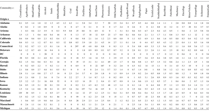
Table 3. Coverage of Census Bureau survey data relative to USAGE-TERM, %a Commodity c: Origin o C er ea lG ra in s A g ri P ro d u ct s M ea tF is h P rd O th F o o d O il s A lc o h o l S an d s O th N o n M et M in M et al O re s C o al P et ro lP rd s F u el D ie se l O th P et P ro d s B asi cC h em P h ar ma ce u ti c F er ti li ze rs O th C h emP rd s P la sR u b b er Lo g sR aw W o o d W o o d P ro d s P u lp P ap er b rd P ap er Te x tl eLe at h r N o n M et M in P rd B ase M et al F ab ri M et al M ac h in er y El ec tr E q p M o to rV eh cl es Tr an sp rt E q p S ci In st rmn t F rn it u re L g h t
Alabama 0.1 0.5 1.4 1.8 12 1.3 4.5 1.2 4.2 1.1 5.8 2.4 3.3 7 30 2.5 2.4 0.1 0.7 0.5 4.4 0.8 1.4 1.1 1 2.8 0.8 0.8 1.4 1.8 0.6 Alaska 0 0.2 2 1.8 0.9 0 0 0 0 4.7 0 2.1 0 0 0 1.7 2.4 0 2.6 0 0 2.1 0.8 12 3.2 11 3.7 20 0.1 3.7 0.7 Arizona 1 0.3 0.6 2.3 3.9 0 0.3 5.9 0.8 25 161 31 6.9 12 0 1 3.1 0.1 0.6 0.3 6.7 2.3 0.4 4.3 0.5 1 0.6 2 2.5 5.8 0.6 Arkansas 3.5 1.3 1 0.6 6.8 0.4 44 0 0 1.3 17 18 12 0.9 23 1.7 0.8 0.1 0.6 0.4 2.1 1.1 1.7 1.1 0.8 1.3 0.5 1.1 12 2 0.3 California 0.6 0.4 0.6 0.9 2.3 0.2 0.4 1.7 0 0.6 9.8 2.1 1.6 1.2 2.3 0.9 0.8 0 1.1 0.3 6.9 1.1 0.6 1.6 0.5 0.8 0.3 0.4 9.2 1.3 0.5 Colorado 0.6 0.3 1.1 1.2 0.7 0.1 0.3 12 0.8 0.5 3.9 1.8 2.1 4.5 14 2.7 1.1 0.1 1.6 0 4.4 0.7 0.5 4.3 1.2 2.5 0.4 1.1 0.5 1.6 0.8 Connecticut 7.2 0.2 0.7 1.3 1.5 0.1 1.6 0 0 297 45 4.8 0.8 0.8 0 0.3 1.3 0 5.4 0.8 6.9 3.3 1.3 9.4 0.5 1.1 1.6 0.8 5.6 1.7 1.1 Delaware 8.4 1.2 0.7 4.9 16 0.4 0 0 0 0 1.8 0.9 0.9 111 0.7 0.7 3.2 0 2.8 0.1 2.5 2.6 1.1 4.1 2.5 10 0.1 0.2 0.9 6.6 1
DC 0 0 0 1 28 0 0 0 0 0 0 0 0 0 0 0.1 0 0 0 0 0 0 1.7 0 1.2 0 0.6 0 0 0 9.4
Florida 28 0.3 0.8 2.1 4.8 0.1 3.2 14 0 18 5.7 1.6 14 5.5 2 3.9 1.9 0 0.9 0.7 3.6 2.5 0.4 3.8 0.5 1.8 1.1 1.6 1.3 2.1 0.7 Georgia 0.2 1.5 0.4 0.6 0.3 0.1 24 0 0 35 13 3.1 3.1 4.1 69 2.5 1.7 0 0.6 0.8 1.3 0.7 1.5 3.2 0.6 2.4 1.1 2.3 4.9 1 0.6 Hawaii 0 0.2 0.5 2.2 5 0.2 1.1 0 0 6.9 0 0 22 167 0 3.2 2.6 0 4.5 0.2 14 13 1.1 0 3.1 43 5.3 10 0 2 1.8 Idaho 2.1 0.6 0.9 2.7 4.8 0.1 0.5 0.1 0 0 0 0 2.4 3.1 5.7 3.3 1.4 0 0.7 1.4 141 1 0.8 3.6 1.2 1.2 0.1 0.9 0.5 4.2 0.5 Illinois 2.8 5.1 1.4 0.8 2.7 1.7 14 0 2.3 2.4 3.7 6 2.8 1.8 0 1.3 0.9 1.4 1.9 0.2 2.4 0.5 0.8 1.5 0.3 0.8 1.2 1 0.9 1.8 0.4 Indiana 2.9 2.1 0.8 2 3.6 0 7.4 0 2.2 2.7 5 1.4 0.7 1.3 0 0.2 0.9 0 1 0.5 3.1 2.6 0.9 0.9 0.3 1.6 0.5 0.3 0.2 0.3 0.5 Iowa 2.5 3.2 1.5 2.1 16 0.8 52 0 0 113 14 35 2 0.4 13 0.7 0.9 0 1.4 0.6 1.9 1.2 0.5 3.7 1 0.6 0.6 2 0.7 1.3 0.4 Kansas 2.6 0.5 1.9 2.1 20 0.1 3.9 0 0 0.2 2.1 4.5 6.2 3.2 48 1.3 1.4 0 4.1 1.6 8 6.4 0.8 37 1.1 1.5 0.9 2.4 1.4 2.1 1.7 Kentucky 1.5 3.4 1.4 0.8 30 0.1 21 217 3.6 3.6 157 7.4 16 115 0 3 1.3 0 1.9 0.6 5.5 6.3 1.9 1.2 0.6 4.1 1.3 0.3 4.2 1.9 1.1 Louisiana 129 30 0.5 1 4 0.5 2.7 0 0 1.6 12 27 1.2 2.5 3.1 0.4 3.1 0.5 0.8 0.4 0.4 5.2 1.5 1.7 1.8 4.5 0.5 0 0.4 8.3 0.6 Maine 3.5 0.2 1.5 1.2 5.8 0.1 84 0 0 59 0 4.2 2.5 2.8 0 15 1.1 0 0.7 0.7 43 2.3 0.8 42 0.3 4.3 1.3 7 0 2.2 0.3 Maryland 1 0.6 0.5 1.9 9.8 0.6 2.4 0 0.4 28 2.9 2.3 1.4 2.5 0.4 2 1.2 0.2 2.1 0.5 2.3 6.3 1.2 1.5 0.5 1.6 0.7 0.7 0.9 1.7 3.4 Massachusett 0 2.6 1.1 1.6 5.2 0.1 2 0 0 0 8.2 1.1 2.1 2.4 0 2.1 1 0 2.5 1.6 3.4 1.1 0.9 4.1 0.2 0.8 0.3 1.5 0.6 2.5 0.7 Michigan 1.6 0.5 2.1 1.1 1.3 0.1 3.6 0 0 10 14 9.7 2.8 12 0 1.4 0.4 0.1 1.8 0.7 6.7 0.9 1.2 1.9 0.3 5.4 0.8 0.2 0.5 1.8 0.7
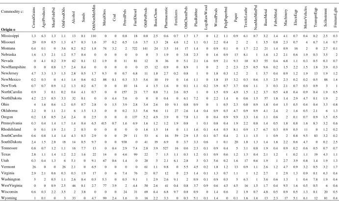
Table 3 (cont.). Coverage of Census Bureau survey data relative to USAGE-TERM, %a
Commodity c:
Origin o C
er ea lG ra in s A g ri P ro d u ct s M ea tF is h P rd O th F o o d O il s A lc o h o l S an d s O th N o n M et M in M et al O re s C o al P et ro lP rd s F u el D ie se l O th P et P ro d s B asi cC h em P h ar ma ce u ti c F er ti li ze rs O th C h emP rd s P la sR u b b er Lo g sR aw W o o d W o o d P ro d s P u lp P ap er b rd P ap er Te x tl eLe at h r N o n M et M in P rd B ase M et al F ab ri M et al M ac h in er y El ec tr E q p M o to rV eh cl es Tr an sp rt E q p S ci In st rmn t F rn it u re L g h t
Mississippi 1.3 6.3 1.3 1.1 13 0.1 110 0 0 0.8 18 0.8 2.5 0.6 0.7 1.7 1.7 0 1.2 1.1 0.9 6.1 0.7 3.2 1.4 4.1 0.7 0.4 0.2 2.5 0.3
Missouri 20 0.9 0.5 1.3 4.7 0.3 1.6 37 0.2 6.5 1.6 3.7 1.3 24 4.6 1.2 1.1 0.1 2.2 0.4 2 2 1 3.5 0.8 2.3 0.7 4 6.7 1.4 0.7
Montana 0.4 0.1 0 3.6 8.2 0.2 1.8 74 3.2 2 722 141 24 3.5 14 17 1.4 0 0.9 0.1 0 1.7 2.2 21 1.4 0.9 16 2 0 2.7 0.1
Nebraska 1.6 1.3 2.1 1.2 5.7 0.4 0 0 0 0 0 0 3 1.9 0 3.8 2.3 0 1.6 0.9 13 8.1 1 1.6 1.2 2.1 0.6 1.9 0.3 3.5 2
Nevada 0 4.1 0.2 3.9 62 0.1 12 1.9 0 11 81 12 8 36 0 5.1 2.1 1.6 0.9 2.1 9.3 10 0.3 55 0.4 6.8 1.1 0.3 0.5 0.3 0.7
NewHampshire 0 0 0.8 1.7 2.4 0.4 0 0 0 0 0 15 12 0.9 0 8.9 1 0 2 2 2.3 2.5 0.5 9.6 0.2 1.5 2.2 1.5 1.8 3.9 0.3
NewJersey 4.7 3.3 1.3 1.5 2.8 0.5 1.7 9.3 0 0.7 6.8 11 1.8 2.7 0.2 0.8 1 0 1.8 0.3 1.2 2 1 3.7 0.4 0.9 1.2 1.9 13 1.9 1.2
NewMexico 0.2 0.3 0 4.1 1.4 0.6 0.2 88 0.1 0.3 3.3 5.6 10 19 0 1.6 1.1 0 1.8 15 3.2 0.3 0.6 1.5 2.5 2.3 0.2 0.2 0.5 88 1.4
NewYork 0.7 0.7 0.9 1.2 1.3 0.2 6.7 0 0 10 14 4 1.5 1.6 0 0.1 1.1 0.2 3.9 0.7 3.7 0.6 1.1 3 0.3 2.1 0.7 0.3 0.9 3 1
NorthCarolin 0.9 3 0.1 0.2 0.4 4.1 0.7 0 0 157 21 7.7 0.8 7.1 3.6 0.5 1 0 1.5 0.9 4.9 1.5 1.2 3.7 0.5 4.8 0.4 0.9 0.4 1.9 0.5
NorthDakota 4.2 2.3 0.5 3.3 32 0.1 0 0 4.4 7.6 0 0 0 0.4 0 6.1 7.2 0 2.2 1.4 6 0.6 1.5 57 1.8 1.4 2.9 4.7 0.1 1.9 2
Ohio 4 1.6 0.6 1.2 0.5 0.7 2.8 0 1.5 3.9 2.8 3.4 2.6 10 9.1 0.8 0.9 0 1 0.5 2.3 0.8 0.9 1.8 0.4 1.5 0.5 0.4 0.4 3.3 0.8
Oklahoma 2.2 0 1.1 2.1 6 1.5 1.3 0 0 0.2 3.3 5.6 9.6 11 27 2.6 1.4 0.4 0.9 0.5 4.7 0.9 0.9 4.1 2.4 2 1.6 0.5 2.1 6 1.3
Oregon 0.2 1.8 0.5 2.4 2.4 0 2.5 0 0 0 137 5.2 4.9 3.9 0 7.8 1.1 0 0.4 0.9 9.9 3.3 1.6 1.1 0.6 2 0.1 0.7 0.9 1.5 0.5
Pennsylvania 0.3 0.4 1.4 1.7 1.4 0.4 6.5 415 0.7 1.6 6.9 1.6 1.2 1.2 1.9 0.8 1 0.1 0.8 0.4 1.9 2.2 0.8 1.4 0.5 1.8 0.8 1.6 8.3 3.2 0.6
RhodeIsland 0 0.1 1.9 2.1 2 0.3 0 0 0 0 0 1.6 1.5 14 0 1.1 1.6 0.1 4.4 0.5 8.1 0.9 1.7 6.7 0.3 0.9 0.5 11 0 1.2 0.2
SouthCarolin 0.6 0.8 1.4 1.4 4.3 0.3 2.9 0 0 29 11 53 6 16 59 2.9 1.5 0.1 0.7 0.4 2 1.1 1.5 1 0.9 2 0.8 9.5 83 3.2 0.2
SouthDakota 2.4 1.5 2.8 18 14 0.5 9.7 0 0 938 0 41 19 6.9 0 3.7 3.3 0.6 1 0.1 20 1.8 1.3 1.4 1.6 2.2 0.6 4.7 0 0.2 2.5
Tennessee 0.8 0.7 1.2 1.1 16 7.7 13 0 0.4 2.9 7.4 2.8 3.9 527 16 0.6 2.3 0.1 0.9 0.4 5 3.1 0.8 1.9 0.4 0.9 0.2 0.6 0.5 0.7 0.7
Texas 2.8 1.1 1.4 1.2 2.2 1.6 22 14 0 4.6 99 22 7 1.5 1.1 0.3 1.2 0.1 0.9 0.6 1.2 1.3 0.4 2.1 1.2 1 0.2 1.1 19 4.3 1.1
Utah 0.3 0.4 1.3 6 5.1 0 9.1 67 0.6 1.4 0 20 5 2.1 6.1 2.8 3 0.3 5.6 0.2 1.6 17 0.6 1.9 1 2.7 3.9 0.8 1.4 1.9 1.3
Vermont 26 0 0 26 2.1 0 6.5 0 0 0 0 61 1.1 9.8 0 5.5 4.5 0.2 1.8 1.2 13 0.9 1.1 2.6 1.2 4.7 0.9 3.2 0.5 3.2 1.7
Virginia 2.9 2.1 0.6 0.3 0.3 1.9 17 0 6 7.4 76 21 0.7 12 0 2.5 1.4 0.1 1.3 0.7 1.1 1 1.2 2.7 1 2.9 1.3 0.9 0.1 6.3 0.4
Washington 5 2 0.5 1.1 2.6 0.4 0.5 5.3 0 0.5 9.1 1 2.9 2.6 9.1 2 0.9 0.1 0.9 0.5 5 6.3 1 3.6 0.6 1.3 1 0.4 7.8 1.9 0.4
WestVirginia 0 0 0.9 2.5 46 0.1 2.7 77 3.9 2 4.4 50 2.6 41 0.4 0.8 3.7 0.9 0.6 4.5 4.5 16 1.5 1.7 0.4 9.5 1.6 0.5 0.5 6 0.6
Wisconsin 0.6 0.3 2.2 3.5 2 3.8 0 0 0 24 31 69 6.4 6.8 9.7 0.8 0.9 0 1.4 0.6 2 1.9 0.7 4.8 0.5 0.9 0.5 1.3 0.1 20 0.5
Wyoming 1 0.1 0 3 33 0 4.7 99 2.4 1.6 0 16 2.2 3.3 0 0.3 5.1 0.1 1.4 0 0.1 1.6 1.6 13 2.3 17 5.1 6.1 12 81 0.4
3. What are the Census Bureau data recording?
3.1 The “sample size” varies widely between commodities and regions
In USAGE-TERM, TRADE(c,o,d) gives us the sales of commodity c from origin o to
destination d. The sum over destinations of an origin’s domestic sales for a given commodity TRADE_D(c,o) is equal to the region’s output of that commodity. The estimates of regional output of each commodity are gathered from a combination of census data, agricultural census data, BEA state level data and other sources.
Let us refer to the corresponding Census Bureau survey data as CFS_TRD(c,o,d) where c is the SCTG commodity shipped from o to d. Similarly, we can sum these Census Bureau data in the destination dimension to obtain CFS_TRD_D(c,o).
The term
Coverage(c,o)= [CFS_TRD_D(c,o)/TRADE_D(c,o)]*100
gives us a measure of the percentage coverage of trade of each commodity by origin.
Let us assume that CFS_TRD_D is a measure of the origin of a commodity (although we will bring this into question). The relevance of this measure is that for small sample sizes, we cannot be confident that the CFS data will provide reliable estimates of the regional
distribution of sales by origin. The larger the Coverage %, the more reliable the estimates are likely to be.
Inspection of the Coverage matrix (table 3) shows that in Alabama, for example, Coverage is as high as 30% for fertilizers and 12% for alcohol. It is less than 0.05% for the agricultural commodity SCTG code 04 (Animal Feed, Eggs, Honey, and Other Products of Animal Origin). If we work through the Coverage matrix, we will find a similar story in other
regions. But what does CFS_TRD_D tell us? Is it really a measure of home state production?
3.2 Transport logistics
The Census Bureau describes the methodology of data collection at
https://www.census.gov/econ/cfs/2012_methodology.html.
The first point to make on the methodology is that it concerns primarily transport logistics. The data concern movements of goods between transport nodes. Tons and ton-miles are the main uses of the data collected, as they are the main determinants of strain on transport infrastructure. Though data on shipment values are collected, they are almost an artefact, perhaps of use to insurers but not the main objective of the survey.
To put the dominance of transport of bulky commodities in the survey into perspective, 50.9% of the total cargo weight recorded in the survey data is accounted for by mining commodities SCTG 10 to 15. They account for 3.9% of total cargo value. Commodities 10 to 15 account for only 0.3% of GDP.
3.3 Data coverage
According to the methodology write-up, the Census Bureau surveys 100,000 out of a
population of 750,000 firms undertaking shipments. The weighted response rate among these 100,000 firms is about 77%. Responders collect data for one week of each quarter of the year.
Second, we can relate the bureau’s estimate of total trade flows to national total production costs. From the USAGE-TERM database, the total costs of production are approximately double GDP. If GDP is $13 trillion, the total costs of production are around $26 trillion. The share of merchandise in total costs is around 22% (i.e., services and utilities account for 78% of total costs, based on the national input-output table), so that total merchandise costs are less than $6 trillion [=0.22*$26 tn]. If we add in merchandise imports which amount to around $1.6 trillion, we expect total merchandise trade flows to be less than $8 trillion. In CGE accounting conventions, we do not double count trade flows. For example, a movement of cargo from A to B to C should be recorded as movement from A to C.
Double counting appears to occur in the Census Bureau’s survey. The first piece of evidence is that the total merchandise trade flow calculated by the bureau of $13.9 trillion far exceeds an estimate we obtain from merchandise costs of production plus imports in a CGE database, which is less than $8 trillion. Other evidence follows, particularly concerning the movement of cereal grains to and through Louisiana.
3.4 What does a trade flow in USAGE-TERM tell us and how does this compare with sample data?
Trade flows in USAGE-TERM tell us of the origin and final regional destination of a commodity. For example, cereal gains produced in Missouri for export from Louisiana appear in the TRADE matrix as a sale from Missouri to Louisiana. The export is recorded in the USE matrix in Louisiana.
The survey data from the Census Bureau record cereal grain shipments through the ports near New Orleans. Inland water shipments from and to New Orleans-Metairie-Hammond of cereal grains are recorded as $256.5 million. Corresponding deep sea shipments from and to New Orleans-Metairie-Hammond ports are $107 million.
Louisiana produces little cereal grain apart from rice. According to the USAGE-TERM database which draws on agricultural census data, Louisiana’s share of national cereal grain production is only 0.8%. Yet the shipments data prepared by the Census Bureau indicate that almost 27% of shipments in the survey data originate from New Orleans ports. What does this mean?
The first point is that the bureau’s sample trade data may but often do not infer a production state of origin (therefore, not all of CFS_TRD_D can be regarded as state production). Moreover, there is the potential for the survey to entail double counting. Missouri which is a substantial producer of cereal grains moves, in the survey data, $170.4 million of cereal grains by inland water ways to the ports of New Orleans. A video on display in the National History Museum of American History on Constitution Avenue, Washington DC, shows how this is done. Grain is poured into hoppers on barges which make their down the Mississippi from the state of Missouri.
After arriving at the barge port in New Orleans, this substantial volume of cereal grains needs to be unloaded. See
https://www.pond5.com/stock-footage/036789596/dry-bulk-cargo-barge-port-new-orleans.html
The ports of New Orleans stretch over 54 miles. A great deal of port activity in the New Orleans region consists of moving cargo from one form of shipping to another. 1 As noted above, $256.5m of cereal grains are moved from one port or mode to another within the New
Orleans region. A further $107m (which arguably could include some the $256.5m) are recorded as deep sea shipping, most likely for export.
The main point of the cereal grains example in the New Orleans region is to show that the inter-regional trade data collected by the Census Bureau for cereal grains bear little relation to the representation of data in USAGE-TERM. The TRADE matrix in USAGE-TERM does not include nodes. The shipment of cereal grains from Missouri to Louisiana appears once in the TRADE matrix, whereas in the bureau’s sample data, it could potentially appear more than once.
Consider the example of Missouri as a destination for cereal grains. In USAGE-TERM, around 75% of cereal-grains destined for Missouri are sourced from within the state. This contrasts with bureau’s sample data in which Missouri is an important transport node for the cereal grains producers deeper into the Mississippi basin, namely Illinois, Iowa, Kansas and South Dakota (Figure 1). Exactly the same transaction as recorded by the bureau may be recorded with a different origin and destination in USAGE-TERM.
A shipment of cereal grains from Iowa to Missouri moved along one of the Mississippi basin’s tributaries may be transferred to a larger barge operated by a different company for the onward journey to New Orleans. This may be recorded as a movement from Iowa to Louisiana. But if it is stored in Missouri for a time before further shipping to Louisiana, it has the potential to contribute to two transactions in the inter-regional trade data. It will
contribute to the bump for Iowa shown in Figure 1. In the bureau’s data, this will not populate the cell for cereal grain originating in Iowa and destined for New Orleans. It will require two nodes, Iowa to Missouri and then Missouri to New Orleans.
In the TRADE matrix of USAGE-TERM, this trade will be recorded as originating in Iowa and destined for New Orleans. In comparing the bureau’s origin shares for shipments into Missouri with those from USAGE-TERM (Figure 1), the bureau’s methodology explains the interstate bumps (green line) and the low own-use share for Missouri relative to the USAGE-TERM TRADE matrix (red line).
Figure 1: Origin shares of cereal grains destined for Missouri in survey data and the USAGE-TERM TRADE matrix
with. For example, we might expect some of South Dakota’s cereal grains output to be exported via Louisiana. South Dakota’s share of total shipments to Missouri is larger in the Census Bureau survey and it share of total shipments to Louisiana smaller than the
corresponding sales shares estimated for USAGE-TERM (Figure 2). These reflect differences in concepts rather than any flaw in the procedure used for allocating inter-regional trades in USAGE-TERM.
Figure 2: Origin shares of cereal grains destined for Louisiana in survey data and the USAGE-TERM TRADE matrix
Figure 3: Destination shares of alcohol originating in California in survey data and USAGE-TERM TRADE matrix
Even so, we note that there is a possible reason for the own-share for California being too low in USAGE-TERM. We might obtain a better fit to Census Bureau data by allocating wine consumption shares by state using
https://www.businessinsider.com.au/wine-consumption-map-united-states-2014-3. The default assumption in USAGE-TERM is that household
consumption shares of each commodity are equal across states. Since California has higher per capita wine consumption than the national average (14 liters per capita compared with less than 11 litres per capita nationally), we expect that its actual own-state sales share is higher than is estimated in USAGE-TERM using the default assumption.
Disaggregated expenditure side data that would enable us to move away from default household consumption shares are not readily available.
3.5 Other examples of excessive “coverage” in the survey data
The example of grain movements in Louisiana is not an isolated case. Table 3 reveals that coverage as defined in footnote a of table 3 for SCTG 17 (gasoline, aviation fuel and ethanol) exceeds 100% in Arizona and Kentucky. SCTG 16 (crude petroleum) exceeds 100%
coverage in Connecticut and Iowa. A similar example for pharmaceutical products (SCTG 21) arises in Delaware, Hawaii and Kansas, and for paper (SCTG 28) in Idaho. In each case, the role of a location as a transport node rather than origin or destination may explain the excessive apparent coverage.
4. What can multi-regional CGE modellers learn from the bureau’s sample data?
There are two possible areas for improvement in the USAGE-TERM trade estimation procedure. These are drawn from Census Bureau data concerning the Mississippi basin.
4.1 Improvements to the TRADE matrix inferred by Census Bureau survey data
distance between upstream states and Louisiana could be scaled to smaller effective distances so as to shift the allocation of trades for origins within the basin towards destinations within the basin.
4.1.1 Selection of margins
The default assumption in the TERM approach is that a given industry has an identical production technology or cost structure in all regions. When this is not so, the standard action is to disaggregate. Therefore, we have separate hydro-electric generation and coal generation electricity sectors in USAGE-TERM to distinguish between the differences in generation in California and West Virginia.
As noted above, the Census Bureau’s sample data demonstrate the importance of water transport for agricultural products, energy products and chemical products in the Mississippi basin. The corresponding commodities originating or being used elsewhere in the country are less reliant on water transport.
In order to make the decision on appropriate allocations of water transport and other transport margins to various commodities, the Census Bureau’s survey data indicates the two digit commodity groups of relevance. The obvious response to the known differences in modes of transport between the Mississippi basin and elsewhere is to split industries/commodities covering agriculture, energy products and chemical products into two in the national CGE database. For example, Wheat in the existing national CGE database would become Wheat-basin and Wheat-rest. Water transport would be an important margin in sales of Wheat-basin, but in Wheat-rest, its use would approximate zero. Rail transport would be relatively
important in sales of Wheat-rest, less so in Wheat-basin.
Soybeans are another farm commodity that has already been split in the national CGE database from the standard NAICS sectors. 96% of national soybean production is in the Mississippi basin. Soybean sales would require modification to reflect a higher reliance on water transport and a lower reliance on rail transport than is the case for other farm outputs.
5. Concluding remarks
The Census Bureau survey does not provide any evidence that the Horridge gravity formula is invalid. However, the survey data point to water transport being used more and rail transport being used less in the Mississippi basin than elsewhere to ship agricultural, mining and fuel products. This difference can be accommodated by allocating transport margins to sales of a subset of commodities in future database preparation.
In addition, the distance matrix used in the gravity formula that allocates inter-regional trades in USAGE-TERM could be adjusted. For commodities using inland water transport,
distances between pairs of regions in the Mississippi basin could be reduced when applying the gravity formula.
Consider a change in trade policy which affects state A. To get complete picture of regional effects, we want the links between state A and state B to be justifiable. One way might be to do some sensitivity analysis on the Horridge formula. If we focus on a particular trade policy, we would like to check whether variations in the Horridge formula change likely regional outcomes.
References
Dixon, P. and Jorgenson, D. (eds), Handbook of computable general equilibrium modeling. North-Holland, Amsterdam, pp 553–657.
Dixon, P., Rimmer, M. and Wittwer, G. (2011), “Saving the Southern Murray-Darling Basin: the Economic Effects of a Buyback of Irrigation Water”, Economic Record, 87(276): 153-168.
Horridge, M. (2012), “The TERM model and its database”, in Wittwer, G. (ed.), Economic Modeling of Water: the Australian CGE Experience, Springer, Dordrecht, pp. 13-35. Horridge, M, Madden, J. and Wittwer, G. (2005), “Using a highly disaggregated multi-regional single-country model to analyse the impacts of the 2002-03 drought on Australia”,
Journal of Policy Modelling 27(3):285-308, April.
Wittwer, G. and Horridge, M. (2010), “Bringing Regional Detail to a CGE Model using Census Data”, Spatial Economic Analysis, 5(2):229-255.