The Utility of Data Transformation for Alignment, de novo Assembly and Classification of Short Read Virus Sequences

(1)

Article Paper

1

The utility of data transformation for alignment, de

2

novo assembly and classification of short read virus

3

sequences

4

Avraam Tapinos1,*_{, Bede Constantinides}1,3_{, My VT Phan}2_{, Samaneh Kouchaki}1,4_{, Matthew Cotten}2_,

5

and David L Robertson1,5

6

1_{School of Biological Sciences, The University of Manchester, Manchester, UK}

7

2_{Department of Viroscience, Erasmus Medical Centre, Rotterdam, the Netherlands}

8

3_{Nuffield Department of Medicine, University of Oxford, Oxford, UK}

9

4_{Department of Engineering Science, University of Oxford, Oxford, UK}

10

5_{MRC-University of Glasgow Centre for Virus Research, Glasgow, UK}

11

12

* Correspondence [email protected]; Tel.: +44 (0) 161 701 7563

13

Received: date; Accepted: date; Published: date

14

Abstract: Advances in DNA sequencing technology are facilitating genomic analyses of

15

unprecedented scope and scale, widening the gap between our abilities to generate and fully exploit

16

biological sequence data. Comparable analytical challenges are encountered in other data-intensive

17

fields involving sequential data, such as signal processing, in which dimensionality reduction (i.e.,

18

compression) methods are routinely used to lessen the computational burden of analyses. In this

19

work we explore the application of dimensionality reduction methods to numerically represent

20

high-throughput sequence data for three important biological applications of virus sequence data:

21

reference-based mapping, short sequence classification and de novo assembly. Despite using highly

22

compressed sequence transformations to accelerate the processes, our sequence processing approach

23

yielded comparable accuracy to existing approaches, and are ideally suited for sequences originating

24

from highly diverse virus populations. We demonstrate the application of our methodology to both

25

synthetic and real viral pathogen sequence data. Our results show that the use of highly compressed

26

sequence approximations can provide accurate results and that useful analytical performance can be

27

retained and even enhanced through appropriate dimensionality reduction of sequence data.

28

Keywords: Alignment, assembly, taxonomic classification, time series, data transformation, DWT,

29

DFT, PAA, data compression, compressive genomics

30

31

1. Introduction

32

Next generation sequencing (NGS) enables massively parallel determination of nucleotide

33

order within genetic material, making it possible to rapidly sequence the genomes of individuals,

34

populations and metagenomic samples [1-5]. However, the sequences generated by these

35

instruments are almost always considerably shorter in length than the genomic regions studied.

36

Genomic analyses often begin with the process of sequence assembly, where sequence fragments

37

(reads) are reconstructed into the larger sequences from which they originated. Computational

38

methods play a vital role in the assembly of short reads, and a variety of assemblers and related tools

39

have been developed in tandem with emerging sequencing platforms [6]. All subsequent analyses

40

and investigations depend upon the quality, accuracy and speed of this crucial sequence assembly

41

process.

42

(2)

There are many computational methods to generate consensus sequences representing the

43

genomes of coexisting species in a sample. Such approaches includes seed-and-extend alignment

44

methods using suffix array derivatives such as the Burrows-Wheeler Transform (BWT) for aligning

45

short reads informed by a known reference sequence [7,8], and graph-based methods employing

46

Overlap Layout Consensus (OLC) [9,10] and de Bruijn graphs of k-mers [11-13] for reference-free de

47

novo sequence assembly. However, for sequencing projects to characterise genetic variation within

48

populations (deep sequencing), metagenomics and pathogen discovery, the effectiveness of the

49

aforementioned approaches varies considerably [14].

50

Samples with mixed viral infections, especially those comprising divergent variants, present a

51

number of analytical and computational problems. The use of a reference sequence, even the use of a

52

data specific generated sequence, can lead to valuable read information being discarded during the

53

alignment process [15]. On the other hand, while de novo approaches require little a priori knowledge

54

of target sequence composition, the methods are computationally intensive and their performance

55

scales poorly with datasets of increasing size [9]. Aggressive heuristics must be employed, to

56

traverse graphs and deal with mismatches, to reduce the running time of de novo assemblers, which

57

in turn can compromise assembly quality. Indexing structures such as the BWT and FM-index are

58

widely used to reduce the burden of pairwise sequence comparison, for both reference base

59

mapping and de novo assembly. However, they cannot process mismatches within reads,

60

necessitating the use of aggressive and computationally expensive heuristics to establish

61

relationships on divergent reads. The increasing NGS read length will affect the performance of

62

these approaches [16].

63

A major challenge working with high-throughput sequencing data for metagenomics and

64

within-host variation analysis is the substantially great diversity of biological data. Also the amount

65

of sequences generated challenge many computational system for a feasible working solution in

66

terms of time and the computational resources typically available in biological laboratories. For

67

biologists working in outbreak responses or pathogen discovery, both the accuracy of the assembly

68

results and the speed of sequence analyses (e.g. assembly, alignment and pathogen classification) are

69

crucial for crisis response and management. The ability to run analyses in the field on portable

70

computer systems without internet connectivity is also important. Here, we explore the utility of

71

data transform methods (used in data intensive fields such as signal and image processing) to extract

72

major features from viral NGS sequence data and use the features to analyse data in a lower

73

dimensional space.

74

Similar analytical challenges involving high dimensional sequential data are encountered in

75

other data-intensive fields such as signal and image processing, and time series analysis, where data

76

transforms and approximation techniques are used for data dimensionality reduction. Data

77

transform/approximation techniques include the discrete Fourier transform (DFT) [17], the discrete

78

wavelet transform (DWT) [18,19], and piece-wise aggregate approximation (PAA) [20,21]. The DFT

79

or DWT are used to transform data to their frequency domains, allowing feature extraction [22], and

80

PAA is used as a data approximation approach. In data intensive fields, data

81

transformations/approximations are commonly used as dimensionality reduction approaches, for

82

obtaining fast approximate solutions for a given problem. Due to the ordered nature of genetic data,

83

many of these transformation approaches can be applied to sequences of nucleotides [23] or amino

84

acids [24]. An example of a successful implementation of a Fourier transform in computational

85

biology is the alignment algorithm MAFFT [25] where the physiochemical properties of amino acids

86

are used to represent sequences for fast matching of homologous sequence regions for alignment.

87

Since most transformation approaches are suitable only for numerical sequences, the strings of

88

letters representing genetic sequences must be mapped into numerical space using a numerical

89

sequence representation method [26].

90

In addition to the DFT, the DWT and PAA, suitable methods for measuring the pairwise

91

similarity of sequential data or transformations include the Lp-norms [27], dynamic time warping

92

(DTW) [28], longest common subsequence (LCS) [29] and alignment approaches such as the

93

(3)

widely used Lp-norm method for sequential data comparison but can only be used on sequences

95

with same lengths. Furthermore, Lp-norm methods do not accommodate shifts in the x-axis (time or

96

position) and are thus limited in their ability to identify similar features within offset data. Elastic

97

similarity/dissimilarity methods such as LCS, unbounded DTW and various alignment algorithms

98

permit comparison of data with different dimensions and tolerate shifts in the x-axis. These

99

properties of elastic similarity methods can be very useful in the analysis of speech signals, for

100

example, but can be computationally expensive [30]. Several approaches have been proposed to

101

permit fast search with DTW, including the introduction of global constraints (wrapping path) or the

102

use of lower bounding techniques such as LB_keogh [28].

103

While pairwise comparison methods may be used for clustering, classification and similarity

104

searches, they are very time consuming for large datasets (O(n2) time complexity). Indexing

105

structures such as the R*-tree, KD-tree, VP-tree and MVP-tree have significantly lower time

106

complexity (O(n log(n))) for similarity search [31] and are more appropriate for efficient analysis of

107

large datasets. The R*-tree [32,33] and KD-tree [34] indexing structures are very accurate for low

108

dimensional datasets. However, their performance deteriorates significantly in high dimensional

109

space [31], known as the ‘curse of dimensionality’ [35,36]. Metric trees such as the VP-tree [37] and

110

MVP-tree [38] are less prone to this limitation. Metric space indexing structures make use of

111

geometric properties for partitioning data and work efficiently on both low and high dimensional

112

data [39]. The curse of dimensionality can be further mitigated using data approximations such as

113

the DFT, the DWT, and the PAA to partition a dataset in an approximated space without loss of

114

generality [21].

115

Here we investigate the performance of three established dimensionality reduction techniques,

116

on three common analysis tasks involving viral short read sequence data: classification, reference

117

based mapping/alignment, and de novo assembly. We benchmarked the accuracy of our proposed

118

methodology against existing tools, and demonstrated the applicability of time series and signal

119

processing data mining techniques for the analysis of viral NGS data.

120

2. Materials and Methods

121

2.1. Symbolic to numeric sequence representations

122

Various numeric sequence representation methods can be used for symbolising a nucleotide

123

sequence to a numerical space (see Table 1). Depending on the chosen numerical representation,

124

each nucleotide is associated with a specific numerical value or vector. The specific values are

125

assigned to the position of each nucleotide indicating the presence of a nucleotide at each sequence

126

position (Equation 1). Ri is the indicator for a specific nucleotide in the ith position of the sequence S

127

with a length of n nucleotides. Values v1…v5 correspond to the numerical value or numerical vector

128

associated with each nucleotide.

129

(1)

130

131

Methods such as the electron-ion interaction pseudo potentials (EIIP) [40] and the atomic

132

representation approach [41] aim to mimic the biochemical properties of nucleic acids, but introduce

133

some mathematical bias that does not exist in reality [26]. Other methods, like the Voss indictor [42]

134

and the Tetrahedron approach, do not introduce internucleotide mathematical bias, meaning the

135

pairwise distances between each non-identical transformed nucleotide is the same (for example, the

136

otherwise

ì

í

ï

î

ï

(4)

Furthermore, the cumulative sum of a numerical representation R can be used to indicate the

138

trajectory of a sequence in nucleotide space. Table 1 indicates the associate values used for different

139

representation methods [26].

140

2.2. Sequence Transformation

141

Effective methods for transforming/approximating sequential data should: i) accurately

142

transform/approximate data without loss of useful information, ii) have low computational

143

overheads, iii) facilitate rapid comparison of data, and iv) provide lower bounding—where the

144

distance between data representations is always smaller than or equal to that of the original

145

data—guaranteeing against false negative results [43]. We employ the DFT and the DWT

146

transformation methods and PAA approximation method as they satisfy the above requirements,

147

are widely used for analysing discrete signals [44], and can be used to transform/approximate

148

nucleotide sequence numerical representations to different levels of resolution, permitting reduced

149

dimensionality sequence analysis.

150

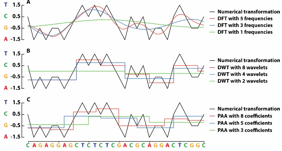
Figure 1A illustrates an example of the DFT and DWT transformations and PAA approximation

151

of a short nucleotide sequence. DFT and the fast Fourier transform (FFT) transform data from their

152

original domain to a frequency domain. In principle, the DFT decomposes a numerically represented

153

nucleotide sequence with n positions (dimensions) into a series of n frequency components ordered

154

by their frequency. A subset of the resulting Fourier frequencies are used to approximate the original

155

sequence in a lower dimensional space [17], and the tradeoff between analytical speed and accuracy

156

can be varied according to the number of frequencies considered [45]

157

DWT transform data from their original domain to their time-frequency, accommodating for

158

changes in signal frequency over time [18,46,47]. DWT is a set of averaging and differencing

159

functions that may be used recursively to represent sequential data at different resolutions and each

160

resolution can be used as an approximation of the original data. Figure 1B depicts an example of the

161

DWT transformations of a short nucleotide sequence.

162

In PAA a numerical sequence is divided into n equally sized windows, the mean values of

163

which together form a compressed sequence representation [20,21]. The selection of n determines the

164

resolution of the compressed or approximate representation. While PAA is faster and easier to

165

implement than the DFT and the DWT, unlike these two methods it is irreversible, meaning that the

166

original sequence cannot be recovered from the approximation. Figure 1C depicts an example of the

167

PAA transformations of a short nucleotide sequence.

168

2.3. Similarity search approaches for sequential data

169

Here we adopt the Euclidian distance and VP-indexing tree to partition our data based on their

170

approximate space distances and perform a fast k-nearest neighbor (k-NN) similarity search for

171

aligning the reads to the reference genome.

172

In a VP-tree indexing structure, data partitioning is implemented in metric space. A data point

173

which is used as a vantage point is selected (either randomly or by applying some heuristic to find

174

and use the furthest point in the dataset [37]), and the rest of the data points are partitioned into two

175

nodes based on their distance to that point. Data found to be closer to the vantage point than a given

176

threshold (the median distance between all the data points and the vantage point) are assigned to the

177

same node, and the rest of the data points to a different node. This function is repeated recursively in

178

order to complete the partitioning process. The resulting indexing structure can then be used for fast

179

identification of a k-nearest neighbour (k-NN) search. A k-NN-search returns the data points that are

180

closest to a query q. Initially, the distance between the query q and the vantage point in the top node

181

is calculated. If the distance between q and the vantage point satisfies a set of given conditions (the

182

distance is smaller or larger than a given threshold – this threshold being the median distance

183

between the vantage point and other data points within the node), a decision is made to visit either

184

one or both of the nodes. This process is repeated until the entire tree has been traversed. The k data

185

points—in this case reads— found closest to our query are the k-nearest neighbours to the query q.

186

(5)

2.4. Proposed short reads processing methodology

188

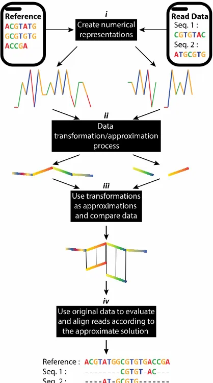
Our methodology for taxonomic classification, reference based mapping and de novo assembly

189

of short reads, used time series and digital signal processing data transformation techniques. Figure

190

2 illustrates the fundamental concept of our approach. The short reads and reference genomes are

191

mapped to a numerical space using an appropriate method from table 1. Subsequently, lower

192

dimensional approximations are generated for all data using the appropriate data transformation

193

method, such as DFT, DWT, and PAA. A VP-tree is constructed to allow fast data comparison.

194

Depending on the application, the VP-tree is constructed either by using k-mer transformations

195

obtained from the reference genomes or by using the short reads’ transformations. Consequently,

196

the best matches for our short reads’ transformations are identified using a k-NN search approach on

197

the VP-tree. As a final step, the results obtained from the k-NN search are re-evaluated in the original

198

space to remove potential false positive results.

199

2.5. Data

200

The implementations of our proposed methodologies were assessed with both simulated and

201

real virus datasets. The simulated datasets were generated using CuReSim [48] and WGSIM

202

(https://github.com/lh3/wgsim ). Simulated data included information such as the reference genome

203

used, the alignment position, and alignment direction for each read, enabling rigorous evaluation of

204

the proposed techniques. We used two simulators to generate different datasets to test our approach

205

under every eventuality. CuReSim can generate long Ion Torrent reads, allowing the user to control

206

the type of variation (insertion, deletion and substitution) to simulate. The user can also define the

207

extent of variation for each individual type of variation. WGSIM can simulate diploid genomes with

208

uniform insertion, deletion and substitution sequencing variation.

209

CuReSim was used to generate 16 HIV-HXB2 simulated datasets with different levels and

210

types of variation. WGSIM was used to generate 4 mixed virus datasets with different levels of

211

variation. Each simulation contained 200,000 reads generated using 5 Norovirus genomes, 5 Ebola

212

virus genomes, and 5 Respiratory syncytial virus (RSV) genomes, with various types and extents of

213

simulated variation. Table 2 contains detailed information about the simulated datasets.

214

Furthermore, 15 publicly available real virus datasets were used for the evaluation of our

215

methodology. The real datasets comprise 5 Norovirus, 5 Ebola virus, and 5 human respiratory

216

syncytial virus (RSV) short read datasets. Norovirus NGS datasets (ERR225628, ERR225629,

217

ERR225631, ERR225632, ERR225633) were generated from diarrhoeal patients in Vietnam [49].

218

Group A rotavirus datasets were obtained from human and pig samples from Vietnam [50]. Human

219

coronavirus NL63 datasets were obtained from Kenya [51]. The Ebola virus datasets (SRR3107337,

220

SRR3107338, SRR3107340, SRR3107342, SRR3107343) were retrieved from the bioproject

221

PRJNA309162, generated during the outbreaks in West Africa in 2013-2016 [52]. The human

222

respiratory syncytial virus (RSV) datasets, ERR303259, ERR303260, ERR303261, ERR303262,

223

ERR303263 [53], were generated from humans in Kenya. Further information for the real data can be

224

found in Table 3.

225

The HIV-HXB2 genome (K03455) was used as a reference index to align and or run the

226

taxonomic classification analysis for the HIV-HXB2 simulated dataset. The Norovirus genome

227

KM198509, the Ebola virus genome KM034562, and the RSV genome KP317934, were used as a

228

reference index to align and or run the taxonomic classification analysis for the mixed virus datasets.

229

The Norovirus genome KM198509 was used to run the taxonomic classification analysis on the real

230

Norovirus datasets, the Ebola virus genome KM034562 was used to run the taxonomic classification

231

analysis on the real Ebola datasets, and the RSV genome KP317934, was used to perform the

232

taxonomic classification analysis on the real RSV datasets. Further information for the reference

233

genomes can be found in Table 4.

234

(6)

The accuracy of a classification and an alignment tool can be quantified in terms of F-measure

236

[48], a balanced measure of precision and recall. With precision = true positive/true positive + false

237

positive and recall = true positive/true positive + false negative, then F-measure = 2 x (precision x

238

recall)/ (precision+recall) [48]. In the case of simulated data, information concerning the position of

239

the read on the reference and alignment direction can be used to establish the correctness of an

240

alignment, and thereby provide a more informative F-measure score. Unclassified reads are

241

considered a false negative result. Any hit on the correct section of the genome and in the correct

242

direction report is considered a true positive result. However, if the alignment position and direction

243

information are not available, the F-measure can be calculated from the number of hits reported for a

244

read, or the absence of a hit. Again, unclassified reads are considered false negative results, and

245

classified reads are considered true positive results. In the case of mixed genome data, the F-measure

246

score can be calculated by taking in consideration the number of hits that were reported for a read,

247

as well as if a read was assigned to a reference genome from the same family. If a read is assigned to

248

a genome from a different virus family, it is considered a false positive result, and unclassified reads

249

are considered a false negative result.

250

3. Results

251

3.1. Classification by numbers (CBN)

252

For the taxonomic classification analysis, a classification tool was implemented in C++

253

(https://github.com/Avramis/ClassificationByNumber). The implementation was developed to

254

evaluate our methodology but is not optimised for speed. Users may specify parameters such as the

255

representation method, transformation method, search stringency and the k-mer length. A

256

vantage-point tree (VP-Tree) indexing structure, containing information from a set of given genomic

257

references, is used to classify reads. The initial step to build the VP-Tree is to extract all of the unique

258

k-mers, of a user-specified size k, from a set of given reference genomes. Each unique k-mer is

259

represented in numerical sequence, and then transformed to a lower dimensional space. The

260

transformed data are then used to generate the VP-Tree indexing structure. Subsequently, each short

261

read from a query set is converted into numerical space and transformed to a lower dimensional

262

space and evaluated against the VP-tree. The approximate solution is then evaluated using the

263

original data to identify false positive results. The CBN algorithm generates two output files. The

264

first output is a text file providing detailed information on all of the classification hits generated for

265

each read. The information generated for each classification includes the reference name, the

266

direction in which the query read was aligned to the reference, the start and end position of the

267

query on the refence, the alignment score, the CIGAR string, and the actual alignment of the query

268

read on the refence genome. The second output file provides a brief review of the alignment. In

269

every line, it contains the short read’s name, the number of classifications generated for that

270

particular read, the highest classification score obtained, the name of the reference which provided

271

the highest classification score, the alignment direction and starting position on the reference.

272

The CBN tool was evaluated against NCBI-BLAST 2.8.1 BLASTn [54] and Kaiju 1.6.3 [55]

273

classifier tools. BLASTn performs the analysis in nucleotide space, whereas Kaiju translates

274

nucleotide sequences into every possible protein frame and performs the analysis in protein space.

275

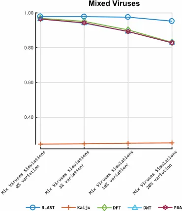
Figures 3, 4, and 5 illustrate the results of the classification evaluation process. Figure 3 shows the

276

results obtained from the classification process on the HIV-HXB2 data. Figure 4 illustrates the results

277

of the mixed virus datasets, and Figure 5 illustrates the results obtained from the real data.

278

In the taxonomic classification of HIV-HXB2 simulated data, where the short reads were

279

classified against the genome that was used to generate them, Kaiju reported the highest accuracy

280

scores. CBN outperformed BLASTn in most cases and only following behind in on the high variation

281

rates datasets. For the mixed viruses simulated datasets, where reads where classified against

282

species strains related to the ones used to generate the reads, BLASTn manage to correctly classify

283

data to the correct species, followed closely by CBN, and Kaiju falling last. In the evaluation of the

284

(7)

species, CBN generated more accurate results compared to the other tools, followed by Kaiju, and

286

BLASTn in third.

287

3.2. Alignment by numbers (ALBN)

288

To test the applicability of sequential data transformations and feature selection for read

289

alignment, we implemented a prototype k-NN read aligner (Table 5) in C++ (available at

290

https://github.com/Avramis/Alignment_by_numbers). As with the CBN classification analysis, the

291

ALBN code was not optimised for speed, and users may specify parameters such as the

292

representation method, transformation method, search stringency and the k-mer length used for

293

seeding alignments. The algorithm’s output was used to construct gapped alignments in the widely

294

used Sequence Alignment/Map (SAM) file format.

295

The ALBN tool was evaluated against a set of well established, widely used, stated of the art

296

tools such as, bowtie2 (version 2.3.1) [56], BWA-MEM (version0.7.16) [7], Graphmap (version 0.5.2)

297

[57], and Segmehl (version 0.3.4) [58]. Each aligner’s accuracy was quantified in terms of F-measure

298

[48]. CuReSim provides information such as the simulated read’s origin on the reference genome

299

and its alignment direction, enabling evaluation of each aligner’s output an calculation of alignment

300

accuracy in terms of F-measure. For mixed virus datasets, tool performance was evaluated in terms

301

of ability to match and align reads to the appropriate virus reference genome. For the real data,

302

F-measures were calculated according to the number of reads aligned to the given genome or

303

otherwise.

304

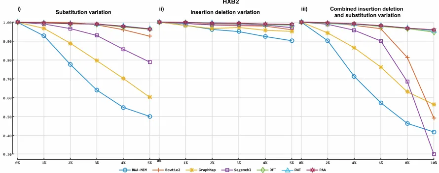
Figures 6, 7 and 8 illustrate the F-measures obtained by evaluating alignments from each

305

aligner. Figure 6 illustrates alignment performance for each of the 16 datasets simulated using the

306

K03455 HIV-HXB2 reference genome. Figure 7 illustrates alignment performance for virus reads

307

simulated with Norovirus genome KM198509.1, Ebola genome KM034562.1, and the RSV genome

308

KP317934.1. Figure 8-i to 8-iii illustrates alignment performance (F-measure) for alignments of real

309

Norovirus, Ebola virus and RSV sequences against the same corresponding reference genomes used

310

in the simulations.

311

ALBN provided highly accurate results in all data cases. Regarding the HIV-HXB2 data, where

312

the short reads were aligned to genome that was used to generate them, ALBN provided the most

313

accurate results in all 16 cases, followed by Bowtie2 in terms of accuracy. Also, in the case of the

314

mixed virus datasets, where reads were aligned against genome strains related to those used to

315

generate the dataset, ALBN provided the most accurate results, with Graphmap and BWA-MEM

316

third and fourth respectively. ALBN also generated the most accurate alignment results using real

317

data, where reads where aligned against a species-specific reference genome.

318

3.3. De novo assembly by numbers

319

Lastly, to test the applicability of this approach to the de novo assembly of short reads, we

320

implemented a naïve algorithm for all-against-all k-mer comparison using data

321

transformations/approximation. Figure 9 illustrates the main concept of our de novo assembly

322

approach. For the ASBN tool, reads are represented as numerical sequences using an appropriate

323

numerical representation method (Table 1). Here we use the tetrahedron numerical representation

324

approach. Every k-mer of each numerically represented read is identified and transformed to lower

325

dimensional space using the chosen transformation method. All k-mers’ transformations are used to

326

build a VP-tree, to allow for fast data comparison. Afterwards, all k-mers are compared to the rest of

327

the data using the VP-tree index. Information from the data comparison is used to construct a

328

weighted graph similar to that shown in Figure 9A. The shortest path on the weighted graph is

329

identified with a breadth-first search (BFS) (Figure 9B). Reads overlaps are used to generate an OLC

330

alignment of short reads (Figure 9C).

331

The ASBN assembler was compared with Megahit (version 1.1.3) [59], and SPAdes (version

332

3.13.0) [60] de novo assemblers on the HIV-HXB2 and mixed virus simulated datasets accordingly.

333

The derived contigs from each assembler were evaluated against the reference genomes used to

334

(8)

and plotted in a histogram. Secondly, a measure of assembly progress was plotted on an X-Y matrix

336

with X being the total coverage of the genomes generated and Y being the total number of gaps in

337

the coverage. A perfect assembly would have X = full genome length and Y = 0, implicating, that the

338

contig matches the genome in terms of size and nucleotide sequences, without any mismatches or

339

gaps. For the HIV-HXB2 datasets, the contigs were evaluated against the K03455 genome, and the

340

contigs obtained from the mixed virus datasets were evaluated against the 15 different genomes,

341

KM198529, KM198528, KM198511, KM198500, KM198486, KU296608, KU296553, KU296549,

342

KU296528, KU296416, KP317952, KP317946, KP317934, KP317923, and KP317922.

343

Figure 10 illustrates the assembly results of SPAdes, Megahit and all three variants of ASBN on

344

the 16 simulated HIV-HXB2 datasets, and Figure 11 illustrates the assembly results on the mixed

345

virus simulated databases. Although ASBN processes data and assembles short reads in a lower

346

dimensional space, it nevertheless generated contigs that collectively cover the expected genome

347

length and provided comparable results to both state of the art de novo assemblers in this

348

experiment(Figure 10, Figure 11). In all cases, ASBN generated contigs spanning the whole genomes

349

of their respective viral species.

350

4. Discussion

351

Although well-established data compression methods for reversible compression of

352

one-dimensional and multivariate signals, images, text and binary exist [61-63]; there are very few

353

examples of their application to biological sequence data. We developed algorithms incorporating

354

signal compression methods for three common biological sequence analysis problems: classification,

355

alignment and de novo assembly of NGS short read virus data. Our results show that our approach

356

permits accurate classification and reference alignment in spite of high rates of sequence variation or

357

the use of a divergent reference genome. Data approximation/summarisation techniques such as the

358

DFT, the DWT and the PAA can be used to extract major features of sequence data and to suppress

359

noise or low-level variation. This allows data comparison in terms of major characteristics, thus

360

enabling the identification of similarities among data that might otherwise be concealed by minor

361

variation or noise.

362

Collectively these results demonstrate that complete nucleotide-level sequence resolution is not

363

a prerequisite of accurate sequence analysis, and that analytical performance can be preserved or

364

even enhanced through appropriate dimensionality reduction (compression) of sequences. While

365

our implementations use k-mers, the nature of the transformation/compression methods used

366

showed that optimal k-mer selection is far less important than with conventional exact k-mer

367

matching methods. The inherent error tolerance of the approach also permits use of larger k values

368

than are normally used with conventional sequence comparison algorithms, reducing the

369

computational burden of pairwise comparison, and thus, in de novo assembly specifically, the

370

complexity of building and searching an assembly graph.

371

Efficient mining of terabase-scale biological sequence datasets requires looking beyond

372

substring-indexing algorithms towards more versatile methods of compression for both data storage

373

and analysis. The use of probabilistic data structures can considerably reduce the computer memory

374

required for in-memory sequence lookups at the expense of a few false positives, and Bloom filters

375

and related data structures have seen broad application in k-mer centric tasks such as error

376

correction [64], in silico read normalisation [65] and de novo assembly [66,67]. However, while these

377

hash-based approaches perform well on datasets with high sequence redundancy, for large datasets

378

with many distinct k-mers, large amounts of memory are still necessary [65]. Lower bounding

379

transformations and approximation methods (such as the DFT, the DWT and PAA) can exhibit the

380

same attractive one-sided error offered by these probabilistic data structures, but instead of hash

381

tables use concrete and thus reusable sequence representations.

382

Furthermore, transformations allow compression of standalone sequence composition,

383

enabling flexible reduction of sequence resolution according to analytical requirements, so that

384

redundant sequence precision need not hinder analysis. While the problem of read alignment to a

385

(9)

formidable problem in computing. Moreover, consideration of the metagenomic composition of

387

mixed biological samples, as demonstrated, further extends the scope and scale of the assembly

388

problem beyond what is tractable using conventional sequence comparison approaches. By

389

implementing a reference-based aligner and de novo assembler, we have demonstrated that using

390

compressed numerical representations representa a tractable and versatile approach for

391

reconstructing genomes and metagenomes sequenced with short reads.

392

In conclusion, short nucleotide sequences may be effectively represented as numerical series,

393

enabling the application of existing analytical methods from a variety of mathematical and

394

engineering fields for the purposes of sequence alignment and assembly. By applying established

395

signal decomposition methods, compressed representations of nucleotide sequences can be created,

396

permitting reductions in the spatiotemporal complexity of their analysis, without necessarily

397

compromising analytical accuracy.

398

399

Authors’ Contribution

400

AT designed and wrote the methods and software, and performed the data analysis with help

401

from BC, MP, SK, and MC. BC and MC, generated the simulated data and BC, MP and MC help on

402

the data evaluation. AT and DLR conceived the study. AT and BC wrote the manuscript with

403

comments from MP, MC and DLR. All authors read and approved the final manuscript.

404

405

Funding

406

This work has been supported by the Wellcome Trust [097820/Z/11/B]; the BBSRC

407

[BB/H012419/1 and BB/M001121/1 and BC by a BBSRC DTP studentship to DLR]; and the

408

VIROGENESIS project which receives funding from the European Union's Horizon 2020 research

409

and innovation programme under grant agreement No 634650.

410

411

412

Figure 1. A numerically represented DNA sequence transformed at various levels of spatial

413

resolution using the discrete Fourier transform (DFT) of the whole sequence (A), the Haar discrete

414

wavelet transform (DWT) (B), and piecewise aggregate approximation (PAA) (C). A 30 nucleotide

415

sequence (x-axis) is represented as a numerical sequence (black lines) using the real number

416

representation method (y-axis where T=1.5, C=0.5, G=-0.5 and A=-1.5) for DFT approximations of the

417

(10)

same sequence with 8 level wavelets (red), 4 level wavelets (blue), and 2 level wavelets (green) (B);

419

and PAA approximations of the same sequence with 8 (red), 5 (blue) and 3 (green) coefficients (C).

420

421

Figure 2. Overview of our proposed methodology using time series transformation/approximation

422

methods: (i) Creation of numerical representations of input sequences. (ii) Application of an

423

appropriate signal decomposition method to transform sequences into their feature space. (iii) Use of

424

approximated transformations to perform rapid data analysis in lower dimensional space. (iv)

425

Validation of inferences against original, full-resolution input sequences. In the case of

426

reference-based alignment, and taxonomic classification, approximated read transformations were

427

compared with a reference sequence. In our de novo implementation, pairwise comparisons were

428

(11)

430

Figure 3. Accuracy of our prototype classification implementation and two established tools on

431

HIV-HXB2 simulated datasets. All plots illustrate the F-measures obtained on the 16 different HIV

432

datasets. The Y axis indicates the F-measure score, and the X axis depicts the reads data files. Plot 3-i

433

depicts the F-measures obtained for each classifier on the simulations with 0% to 5% of substitution

434

variation rate. Plot 6-ii illustrates the F-measures obtained for each classifier on the simulations with

435

0% to 5% uniform insertion/deletion variation and plot 3-iii illustrates the F-measures obtained for

436

each tool on simulations of uniform 0% to 10% insertion/deletion and substitution variation.

437

438

Figure 4. Accuracy of our prototype classification implementation and two established tools on

439

mixed viruses simulated datasets. The Y axis indicates the F-measure score, and the X axis depicts the

440

reads data files. The plot depicts the F-measures obtained for each classifier on the mixed virus

441

simulations.

442

0.90 0.92 0.94 0.96 0.98 1.00

Substitution variation Insertion deletion variation Combined insertion deletion and substitution variation

0% 1% 2% 3% 4% 5% 0% 1% 2% 3% 4% 5% 0% 2% 4% 6% 8% 10% BLAST Kaiju DFT DWT PAA

HXB2

(12)

443

Figure 5. Accuracy of our prototype classification implementation and two established tools on real

444

sequences. The Y axis indicates the F-measure score, and the X axis depicts the reads data files. The Y

445

axis indicates the F-measure score, and the X axis depicts the reads data files. Plot 5-i depicts the

446

F-measures obtained for each classifier on the Norovirus sequences data. Plot 5-ii illustrates the

447

F-measures obtained for each classifier on the Ebola sequence data. Plot 5-iii illustrates the

448

F-measures obtained for each tool on Respiratory syncytial virus (RSV) sequence data.

449

450

Figure 6. Accuracy of our prototype reference alignment implementation and four established tools

451

on HIV-HXB2 simulated datasets. Figure 6 illustrates the F-measures obtained on the 16 different

452

HIV datasets. Plot 6-i depicts the F-measures obtained for each aligner on the simulations with 0% to

453

5% of substitution variation rate. Plot 6-ii illustrates the F-measures obtained for each aligner on the

454

simulations with 0% to 5% uniform insertion/deletion variation and plot 6-iii illustrates the

455

F-measures obtained for each tool on simulations of uniform 0% to 10% insertion/deletion and

456

substitution variation.

457

ERR3 0325

9

ERR3 0326

0

ERR3 0326

1

ERR3 0326

2

ERR3 0326

4

0.20 0.40 0.60 0.80 1.00

RSV

ERR2 2562

8

ERR2 2562

9

ERR2 2563

1

ERR2 2563

2

ERR2 2563

3

0.20 0.40 0.60 0.80

1.00 Norovirus

SRR3 1073

37.1

SRR3 1073

38.1

SRR3 1073

40.1

SRR3 1073

42.1

SRR3 1073

43.1

0.88 0.90 0.92 0.94 0.96 0.98 1.00

Ebola

BLAST Kaiju DFT DWT PAA

i) ii) iii)

0.40 0.50 0.60 0.70 0.80 0.90 1.00

Substitution variation Insertion deletion variation Combined insertion deletion and substitution variation

0% 1% 2% 3% 4% 5% 0% 1% 2% 3% 4% 5% 0% 2% 4% 6% 8% 10%

HXB2

0.30

BWA-MEM Bowtie2 GraphMap Segemehl DFT DWT PAA

(13)

458

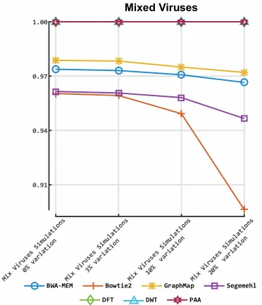
Figure 7. Accuracy of our prototype aligner implementation and four established tools on mixed

459

viruses simulated datasets. The Y axis indicates the F-measure score, and the X axis depicts the reads

460

data files. The plot depicts the F-measures obtained for each aligner on the mixed virus simulations

461

462

Figure 8. Accuracy of our prototype aligner implementation and four established tools on real

463

sequences datasets. The Y axis indicates the F-measure score, and the X axis depicts the reads data

464

files. The Y axis indicates the F-measure score, and the X axis depicts the reads data files. Plot 8-i

465

depicts the F-measures obtained for each aligner on the Norovirus sequences data. Plot 8-ii illustrates

466

the F-measures obtained for each aligner on the Ebola sequences data. Plot 8-iii illustrates the

467

F-measures obtained for each tool on the Respiratory syncytial virus (RSV) sequences data.

468

Mix Viru

ses Simu

lati ons

0% v aria

tion

Mix Viru

ses Simu

lati ons

3% v aria

tion

Mix Viru

ses Simu

lati ons

10% var

iati on

Mix Viru

ses Simu

lati ons

20% var

iati on

0.91 0.94 0.97 1.00

Mixed Viruses

BWA-MEM Bowtie2 GraphMap Segemehl

DFT DWT PAA

ERR2 2562

8

ERR2 2562

9

ERR2 2563

1

ERR2 2563

2

ERR2 2563

3

0.20 0.40 0.60 0.80 1.00

Norovirus

SRR3 1073

37.1

SRR3 1073

38.1

SRR3 1073

40.1

SRR3 1073

42.1

SRR3 1073

43.1

0.84 0.88 0.92 0.96 1.00

Ebola

0.82

ERR3 0325

9

ERR3 0326

0

ERR3 0326

1

ERR3 0326

2

ERR3 0326

4

0.40 0.60 0.80 1.00

Respiratory Syncytial Virus

0.20

BWA-MEM Bowtie2 GraphMap Segemehl DFT DWT PAA

(14)

469

Figure 9. A de novo assembly methodology for numerically represented nucleotide reads.

470

All-against-all sequence comparison (A) enables construction of a read graph with weighted edges.

471

The weight assigned to each edge is the smallest pairwise distance between every possible k-mer

472

representation of the two reads. (B) The shortest path in the graph is identified with a breadth-first

473

search algorithm (red coloured edges) thereby (C) enabling read alignment. A DNA walk

474

representation of the overlapped reads (D) may subsequently be used as a three-dimensional

475

graphical portrayal of the reads, illustrating alignment characteristics.

476

477

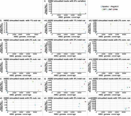
Figure 10. Accuracy of our prototype de novo assembly implementation and two established tools on

478

HIV-HXB2 simulated datasets. The contigs obtained for each assembler were evaluated against the

479

reference genome used to generate the simulated data. BLASTn was used to align all contigs to a

480

0 10 15 20 25

HXB2 genome coverage

HXB2 simualted reads with 2% sub. var .

5 iii)

0 2000 4000 6000 8000

HXB2 simualted reads with 0% variation

0 100 200 300 400 500

0 2000 4000 6000 8000

i) 0.0 2.0 1.5 3.0 2.5 1.0 0.5

HXB2 simualted reads with 1% sub var .

0 2000 4000 6000 8000

ii) G a p s / N s / M i s m a t c h e s

0 2000 4000 6000 8000

400 600 800 1000 0 200

HXB2 simualted reads with 1% indel var . vii)

HXB2 genome coverage 0 2000 4000 6000 8000

700 0 100 200 300 400 500 600

HXB2 simualted reads with 2% com. var. xii)

0 200 400 600 800 1000

1200HXB2 simualted reads with 4% com. var. xiii)

0 2000 4000 6000 8000

G a p s / N s / M i s m a t c h e s 0 200 400 600 800 1000 1200

1400HXB2 simualted reads with 2% indel var . viii) G a p s / N s / M i s m a t c h e s

0 2000 4000 6000 8000

0 5 10 15 20 25 30

HXB2 simualted reads with 3% sub. var. iv)

0 2000 4000 6000 8000

0 2040 60 80 100 120

HXB2 simualted reads with 4% sub. var. v)

0 2000 4000 6000 8000

0 50 100 150 200

HXB2 simualted reads with 5% sub. var. vi)

0 2000 4000 6000 8000

400 800 2000

1200 1600

HXB2 simualted reads with 3% indel var . ix)

0 2000 4000 6000 8000

G a p s / N s / M i s m a t c h e s 2400 800 2000 1200 1600

HXB2 simualted reads with 4% indel var . x)

0 2000 4000 6000 8000

G a p s / N s / M i s m a t c h e s 500 1000 1500 2000 2500 3000

HXB2 simualted reads with 5% indel var . xi)

0 2000 4000 6000 8000

G a p s / N s / M i s m a t c h e s 0 500 1000 1500 2000 2500

0 2000 4000 6000 8000

G a p s / N s / M i s m a t c h e s

HXB2 simualted reads with 6% com.var. xiv) 0 1000 2000 3000 4000 5000

6000HXB2 simualted reads with 8% com.var. xv)

0 2000 4000 6000 8000

G a p s / N s / M i s m a t c h e s 0 2000 4000 6000 8000 10000 12000 G a p s / N s / M i s m a t c h e s

HXB2 simualted reads with 10% com. var . xvi)

0 2000 4000 6000 8000

DFT DWT PAA

(15)

HIV-HXB2 refence genome and determine genome coverage. The Y axis indicates the number of

481

gaps and mismatches that exist in the contigs obtained for each tool, and the X axis depicts the length

482

of the genome the reported contigs cover. The contigs obtained from the assembly of the HIV-HXB2

483

simulated short read data were evaluated against the K03455 reference genome. Plot 10-i illustrates

484

results obtained from all assemblers on variation free data. Plots 10-ii to 10-vi illustrate results

485

obtained from all assemblers on data with different levels of substitution variation. Plots 10-vii to

486

10-xi illustrate results obtained from all assemblers on data with different levels of insertion/deletion

487

variation. Plots 10-xiii to 10-xvi illustrate results obtained from all assemblers on data with different

488

levels of combined insertion/deletion and substitution variation.

489

490

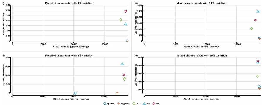
Figure 11. Accuracy of our prototype de novo assembly implementation and two established tools on

491

mixed viruses simulated datasets. The contigs obtained for each assembler were evaluated against

492

the reference genome that was used to generate the simulated data. BLASTn was used to align all

493

contigs to a HIV-HXB2 refence genome, and determine how much of the particular genome they do

494

cover. The Y axis indicates the number of gaps and mismatches that exist in the contigs obtained for

495

each tool, and the X axis depicts the length of the genome the reported contigs cover. The contigs

496

obtained from the mixed virus simulated dataset were evaluated against the, KM198529, KM198528,

497

KM198511, KM198500, KM198486, KU296608, KU296553, KU296549, KU296528, KU296416,

498

KP317952, KP317946, KP317934, KP317923, and KP317922 references genomes. Plots 11-i to 11-iv

499

illustrate results obtained from all assemblers on data with 0%, 3%, 10% and 20% variation levels

500

accordingly.

501

502

G a p s / N s / M i s m a t c h e s

Mixed viruses reads with 0% variation

Mixed viruses genome coverage 0 100 200 300 400 500 600 700

0 5000 10000 15000

G a p s / N s / M i s m a t c h e s 0 500 1000 1500 2000

Mixed viruses genome coverage

Mixed viruses reads with 3% variation

0 5000 10000 15000

G a p s / N s / M i s m a t c h e s 0 500 1000 1500 2000 2500

3000 Mixed viruses reads with 10% variation

0 5000 10000 15000 Mixed viruses genome coverage

G a p s / N s / M i s m a t c h e s 1000 2000 3000 4000

5000 Mixed viruses reads with 20% variation

0 5000 10000 15000 Mixed viruses genome coverage

Spades Megahit DFT DWT PAA

i)

ii)

iii)

(16)

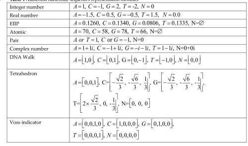
Table 1 Numerical nucleotide sequences representation methods.

503

Integer number

A

=

1,

C

=

-1,

G

=

2,

T

=

-2,

N

=

0

Real number

A

= -

1.5,

C

=

0.5,

G

= -

0.5,

T

=

1.5,

N

=

0.0

EIIP

A

=

0.1260,

C

=

0.1340,

G

=

0.0806,

T

=

0.1335, N=

Æ

Atomic

A

=

70,

C

=

58,

G

=

78,

T

=

66, N=

Æ

Pair

A

or

T

=

1,

C

or

G

= -

1, N=0

Complex number

A

=

1 +

1 i

,

C

= -

1 +

1 i

,

G

= -

i

-

1 i

,

T

=

1 -

1 i

, N=0+0i

DNA Walk

A

=

é

_ë

1,0

ù

_û

,

C

=

é

_ë

0,1

ù

_û

, G

=

_ë

é

0,

-

1 ù

_û

,

T

= -

é

_ë

1,0

ù

_û

,

N

=

é

_ë

0,0

ù

_û

Tetrahedron

A

=

é

_ë

0,0,1

ù

_û

, C=

-

2

3 ,

-6

3 ,

1

3 é

ë

ê

ù

û

ú

, G=

-

2

3 ,

-6

3 ,

-1

3 é

ë

ê

ù

û

ú

,

T= 2

´

2

3 , 0,

-1

3 é

ë

ê

ù

û

ú

, N= 0, 0, 0

é

ë

ù

û

Voss indicator

_A

₌

é

_ë

_0,0,1,0

ù

_û

_,

_C

₌

_ë

é

_1,0,0,0

ù

_û

_,

_G

₌

é

_ë

_0,1,0,0

ù

_û

_,

T

=

é

_ë

0,0,0,1

ù

_û

,

N

=

é

_ë

0,0,0,0

ù

_û

504

(17)

506

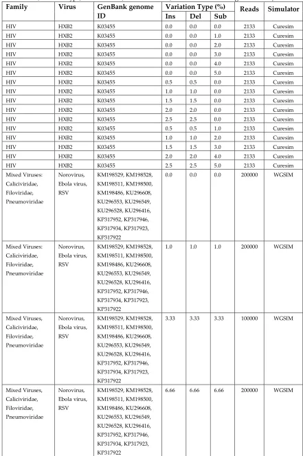
Table 2. Simulated read data. Each row contains details for each simulated dataset (i.e. virus family, virus,

507

GenBank id, variation type, variation level, number of reads, and simulator used to generate data).

508

Family Virus GenBank genome

ID

Variation Type (%) _Reads _Simulator

Ins Del Sub

HIV HXB2 K03455 0.0 0.0 0.0 2133 Curesim

HIV HXB2 K03455 0.0 0.0 1.0 2133 Curesim

HIV HXB2 K03455 0.0 0.0 2.0 2133 Curesim

HIV HXB2 K03455 0.0 0.0 3.0 2133 Curesim

HIV HXB2 K03455 0.0 0.0 4.0 2133 Curesim

HIV HXB2 K03455 0.0 0.0 5.0 2133 Curesim

HIV HXB2 K03455 0.5 0.5 0.0 2133 Curesim

HIV HXB2 K03455 1.0 1.0 0.0 2133 Curesim

HIV HXB2 K03455 1.5 1.5 0.0 2133 Curesim

HIV HXB2 K03455 2.0 2.0 0.0 2133 Curesim

HIV HXB2 K03455 2.5 2.5 0.0 2133 Curesim

HIV HXB2 K03455 0.5 0.5 1.0 2133 Curesim

HIV HXB2 K03455 1.0 1.0 2.0 2133 Curesim

HIV HXB2 K03455 1.5 1.5 3.0 2133 Curesim

HIV HXB2 K03455 2.0 2.0 4.0 2133 Curesim

HIV HXB2 K03455 2.5 2.5 5.0 2133 Curesim

Mixed Viruses: Caliciviridae, Filoviridae, Pneumoviridae

Norovirus, Ebola virus, RSV

KM198529, KM198528, KM198511, KM198500, KM198486, KU296608, KU296553, KU296549, KU296528, KU296416, KP317952, KP317946, KP317934, KP317923, KP317922

0.0 0.0 0.0 200000 WGSIM

Mixed Viruses: Caliciviridae, Filoviridae, Pneumoviridae

1.0 1.0 1.0 200000 WGSIM

Mixed Viruses, Caliciviridae, Filoviridae, Pneumoviridae

3.33 3.33 3.33 100000 WGSIM

Mixed Viruses, Caliciviridae, Filoviridae, Pneumoviridae

(18)

509

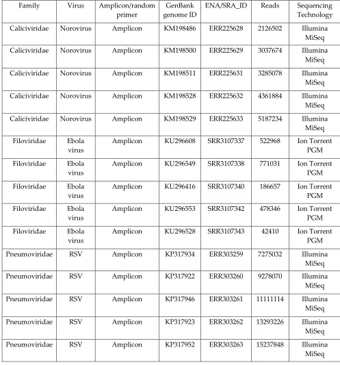
Table 3. Real short reads data. Rows contain information for each real reads’ dataset (i.e. virus

510

family, virus, genome strain GenBank id, SRA project ID, number of reads, and technology used to

511

sequence data).

512

Family Virus Amplicon/random

primer

GenBank genome ID

ENA/SRA_ID Reads Sequencing Technology

Caliciviridae Norovirus Amplicon KM198486 ERR225628 2126502 Illumina MiSeq

Filoviridae Ebola virus

Amplicon KU296608 SRR3107337 522968 Ion Torrent PGM

Pneumoviridae RSV Amplicon KP317934 ERR303259 7275032 Illumina

MiSeq

513

(19)

Table 4. Reference genomes used during classification and reference based alignment

515

Family Virus GenBank id: Length (nt)

Retroviridae Human

immunodeficiency

virus 1

(HXB2)

K03455 9179

Caliciviridae Norovirus KM198509.1 7425

Filoviridae Zaire ebolavirus KM034562.1 18957

Pneumoviridae Human

orthopneumovirus

(Respiratory Syncytial

Virus)

KP317934.1 15233

516

517

Table 5. Pseudocode for the alignment procedure

518

519

520

References

521

1. Margulies, M.; Egholm, M.; Altman, W.E.; Attiya, S.; Bader, J.S.; Bemben, L.A.; Berka, J.; Braverman,

522

M.S.; Chen, Y.-J.; Chen, Z. Genome sequencing in microfabricated high-density picolitre reactors.

523

Nature 2005, 437, 376-380.

524

2. Bentley, D.R.; Balasubramanian, S.; Swerdlow, H.P.; Smith, G.P.; Milton, J.; Brown, C.G.; Hall, K.P.;

525

Evers, D.J.; Barnes, C.L.; Bignell, H.R. Accurate whole human genome sequencing using reversible

526

terminator chemistry. Nature 2008, 456, 53-59.

527

1) Represent short reads and reference genome as numerical sequences. 2) Select k-mer length.

3) Create transformations of each reference sequence k-mer, build VP-tree, and

create transformations of the initial k-mer of each short reads.

4) Identify candidate alignments using data transformations. for each read i

candidate_alignments[i] = VPtree.k-NNSearch(query i) end

5) Align approximate results with original data using the Smith-Waterman (SW)

algorithm:

for each read i best_score = null best_aln = []

for each k neighbour in candidate_alignments[i] if SW_score(k neighbour, read i)

best_score = SW_score(k neighbour, read i) best_aln = SW_aln(k neighbour, read i) end

end end