Algorithm to color a Circuit Dual Hypergraph for
VLSI Circuit
Bornali Gogoi#1, Bichitra Kalita*2
#
Department of Computer Application, Assam Engineering College, Gauhati University
Jalukbari, Guwahati-781013, Assam, India
Abstract— Line-of-sight graph is used to check the number of short circuit testing needed to test a printed circuit board. This paper presents a simple algorithm based on some assumptions to put color in a circuit dual hypergraph of a VLSI circuit. The structures of line-of-sight graphs with 10, 11, 12 and 13 colors have been established. This algorithm can be used to find out number of short circuit testing needed for a VLSI printed circuit board.
Index Terms— Line-of-sight graph, short circuit testing, VLSI circuit, circuit dual hypergraph.
I. INTRODUCTION
Graphs are used in different areas in computer science. Circuit dual hypergraphs are used to represent a circuit using a graph. A special type of these graphs have been represented which shown their possible placement in the printed circuit board [10]. These types of circuit dual hypergraphs are placed in the printed circuit board considering an algorithm [11]. This algorithm has been considered for the planar triangulated graphs. It has been found that the graph coloring is used in many applications like scheduling and assignment problems [3]. An undirected graph G {V, E} can be colored using vertex coloring and edge coloring. A (vertex) coloring of a graph G is a mapping c : V(G) -> S. The elements of S are called colors; the
vertices of one color form a color class. If |S| = k, we say that c is k-coloring (often we use S = {1, …, k). A coloring is proper if adjacent vertices have different colors. A graph is k-colorable if it has a proper k-coloring. The chromatic number c(G) is the least value of k such that G is k-colorable.
Obviously, λ(G) exists as assigning distinct colors to
vertices yields a proper |V(G)|-coloring. An optimal coloring
of G is a λ(G)-coloring. A graph G is k-chromatic if λ(G) = k. Obviously, the complete graph Kn requires n colors, so λ(Kn) = n. Then λ(G) ≥ω(G) where ω(G) is the weight of the
graph G. This bound can be tight, but it can also be very loose. Indeed for any given integers k ≤l, there are graphs
with clique number k and chromatic number l [12]. General
graph coloring algorithms are well known and have been extensively studied by the researchers [5, 6]. A graph has been colored, considering the vertex with minimum degree first [2]. Then the graph considered will contain all the vertices excluding already considered vertex. Many algorithms have been found for graph coloring. Amongst them first fit and degree based ordering techniques are
placed. First Fit algorithm is the easiest and fastest
technique of all greedy coloring heuristics. The algorithm sequentially assigns each vertex the lowest legal color. This algorithm has the advantage of being very simple and fast and can be implemented to run in O(n)[8,9]. Degree based ordering provides a better strategy for coloring a graph. It
uses a certain selection criterion for choosing the vertex to be colored. This strategy is better than the First Fit which simply picks a vertex from an arbitrary order. Some strategies for selecting the next vertex to be colored have already been proposed and remind us as follows:
a.Largest degree ordering (LDO): It chooses a vertex with
the highest number of neighbors. Intuitively, LDO provides a better coloring than the First Fit. This heuristic can be implemented to run in O(n2)[8,9].
b.Saturation degree ordering (SDO): The saturation degree
of a vertex is defined as the number of its adjacent differently colored vertices. Intuitively, this heuristic provides a better coloring than LDO as it can be implemented to run in O(n3)[8,9].
c.Incidence degree ordering (IDO): A modification of the
SDO heuristic is the incidence degree ordering. The incidence degree of a vertex is defined as the number of its adjacent colored vertices. This heuristic can be implemented to run in O(n2)[8,9].
The applications of graph coloring are found in Guarding an Art Gallery, Physical Layout Segmentation, Round-Robin Spots Scheduling, Aircraft Scheduling, Biprocessor Tasks, Frequency Assignment, Map Coloring and GSM Mobile Phone Networks [16, 17] etc. Graph coloring is also used for short circuit testing in VLSI physical design.
II. ALGORITHM TO COLOR A CIRCUIT DUAL GRAPH TO GET A LINE-OF-SIGHT GRAPH
In large PCBs like VLSI, the modules are placed in priority wise while designing them. First few modules placed and connections are made among them. Then they are checked for short circuits. After taking care of the problems arise in this already placed and connected modules, as the next step, few more modules will be placed. Connections will be made among the newly placed modules and the modules placed in the first phase. Again all sorts of testing will be done on this second phase modules including short circuit testing. This process will be repeated phase-wise till
module is utilized to its maximum.
Graph coloring algorithms focused before, as some are stated above, have not been considered the method of coloring for a line-of-sight graph which has been discussed here. Therefore, the number of colors needed to color the line-of-sight graph, as derived by those graph coloring algorithms, will be different from the actual number of short-circuit testing needed in physical design time in VLSI physical design.
Considering this concept, an algorithm has been established to color a circuit dual graph to get the actual number of short-circuit testing needed to design a circuit from it as followings.
A. Algorithm to color the circuit dual graph
Step 1: Consider the priority assigned to the circuits (vertices) of the board (circuit dual graph). Step 2: Place the modules on the board based on priority
basis. Highest priority modules will be placed in the first phase. Connect these modules as desired. Step 3: Put color on these modules accordingly to get the
respective line-of-sight graph. Find out the number of short circuit testing needed.
Step 4: In the second phase, place the next highest priority modules. Repeat step 2 and 3. Total number of short circuit testing needed is same as the number of colors needed for the resulting line-of-sight graph.
Step 5: Repeat step 2 – 4 till all the modules are placed on the board to get the final line-of-sight graph for that circuit dual graph.
Step 6: The total number of colors used to color the circuit dual graph is the actual number of short circuit testing needed to physically design the VLSI circuit. Since it has been known that numerous modules are placed in VLSI printed circuit board. Therefore, it is not possible to place all the modules in one time, to make the connections among them and then test for short-circuit. The VLSI designers opt for a process where they place the modules in phase-wise manner. While using the circuits, designer always utilize one circuit to its optimum level. So, in phase manner, the VLSI designers design the whole board and give them for physical design. Therefore, the total number of short-circuit testing may be different from the number of colors shown by different algorithms placed earlier.
B. Proof:
We are considering the following circuit dual graph G(74, 214) in figure 1 to apply the given algorithm. Numbers given for the vertices are the priority given to each of these modules. Highest priority modules will be placed in the first
Figure 1: A circuit dual graph G (74, 214)
Step 1: The priorities of each of these modules are shown
inside each vertex using numbers. Lower the number higher is the priority.
Step 2: All the modules with priority 1 & 2 are placed on the
board and give the connections as desired.
Step 3: As per the connection, we can place it on the board
and put color in it as shown below in figure 2:
Figure 2: Line of sight graph of figure 1 after placing priority module 1
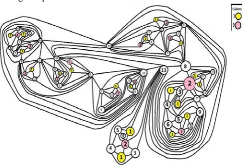
Step 4: The following figure 3 is obtained after going
through step 4.
Step 5:
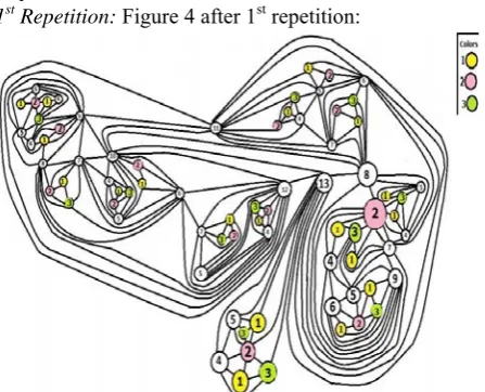
1st Repetition: Figure 4 after 1st repetition:
Figure 4: After placing modules with priority 1, 2 & 3
2nd Repetition: Figure 5 after 2nd repetition:
Figure 5: After placing modules with priority 1, 2, 3 & 4
3rd Repetition: Figure 6 after 3rd repetition:
Figure 6: After placing modules with priority 1, 2, 3, 4 & 5
4th Repetition: Figure 7 after 4th repetition:
Figure 7:After placing modules with priority 1, 2, 3, 4, 5 & 6
5th Repetition: Figure 8 after 5th repetition:
Figure 8:After placing modules with priority 1, 2, 3, 4, 5, 6 & 7
6th Repetition: Figure 9 after 6th repetition:
Figure 9: After placing modules with priority 1, 2, 3, 4, 5, 6, 7& 8
Figure 10: After placing modules with priority 1, 2, 3, 4, 5, 6, 7, 8 & 9
8th Repetition: Figure 11 after 8th repetition:
Figure 11: After placing modules with priority 1, 2, 3, 4, 5, 6, 7, 8, 9 & 10
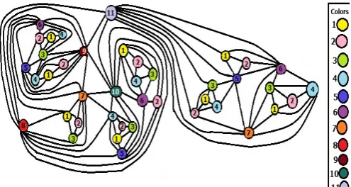
9th Repetition: Figure 12 after 9th repetition:
Figure 12: After placing modules with priority 1, 2, 3, 4, 5, 6 , 7, 8, 9, 10 & 11
Figure 13: After placing modules with priority 1, 2, 3, 4, 5, 6 , 7, 8, 9, 10, 11 & 12
11th Repetition: Figure 14 after 11th repetition:
Figure 14: Line-of-sight-graph with 13 colors
The structure of this graph G(74, 214) is as shown in Figure 15 below.
It is found that the structure of the graph (Figure 15) has 1, 4, 2, 2, 4, 1, 8, 8, 13, 13, 17, and 1 numbers of vertices with degree 13, 12, 11, 10, 9, 8, 7, 6, 5, 4, 3, 2 respectively.
C. Different structures found:
We are finding out the structure of a series of line-of-sight-graph with ten (10), eleven (11) and twelve (12) colors following the assumptions of the above stated algorithm.
i. Line-of-sight-graph with ten (10) colors:
One possible structure of this graph is as in Figure 15a below as G1(27, 74).
Figure 15a: 14 colored line-of-sight-graph It is found that the structure of the graph (Figure 17) has 4, 1, 4, 2, 5, 6, and 5 numbers of vertices with degree 9, 8, 7, 6, 5, 4, 3 respectively.
The structure with mentioning the degree is as shown in Figure 15b G1(27, 74) below.
Figure 15b: 10 colored graph with degree
ii. Line-of-sight-graph with eleven (11) colors:
Line-of-sight-graph with 11 colors is drawn as shown in Figure 16 G2(41, 113) below.
Figure 16: Line-of-sight-graph with 11 colors
The structure of this graph G2(41, 113) is as shown in Figure 17 below.
Figure 17: 11 colored line-of-sight graph with degree of each vertex
It is found that the structure of the graph (Figure 17) has 4, 1, 1, 7, 3, 8, 9, and 8 numbers of vertices with degree 10, 9, 8, 7, 6, 5, 4, 3 respectively.
iii. Line-of-sight-graph with twelve (12) colors:
Line-of-sight-graph with 12 colors is drawn as shown in Figure 18 G3(53, 149) below.
Figure 18: Line-of-sight-graph with 12 colors
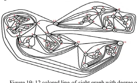
Figure 19: 12 colored line-of-sight graph with degree of each vertex
It is found that the structure of the graph (fig19) has 4, 1, 3, 3, 6, 5, 9, 10, 11, and 1 numbers of vertices with degree 11, 10, 9, 8, 7, 6, 5, 4, 3, 2 respectively.
III. CONCLUSION
This algorithm can be applied to test a VLSI circuit board for short circuit. The difference among the previously established algorithms and this one is the way of placing modules on the board. This algorithm follows phase-wise placement of modules which is practically used to design a VLSI circuit board. So, the number of colors needed to draw the line-of-sight graph in this paper is totally different from the previously established graph coloring algorithms. The above shown structures will need nC
2 number of short circuit testingwhere n is the number of colors used if followed the assumptions as stated above. The same graph may give different color if followed the algorithm discussed in [14]. But considering the process used in designing a board in VLSI, we found these graphs will need 12 or 13 colors as shown in this paper.
Design”, McGraw-Hill International editions, International edition 1996
[2] M. R. Garey, D. Stifler and Hing C. So, “An application of graph coloring to Printed Circuit Testing”, IEEE Transaction on Circuit and Systems, Vol. CAS-23, No. 10, October 1976.
[3] Meena Bharti and Sahil Singla, “Review of Graph Coloring and its Applications”, International Journal of Applied Engineering Research, ISSN 0973-4562 Vol.7 No.11, 2012.
[4] A web link last modified on 3 Sept 2012 at 06:59
http://en.wikipedia.org /wiki/ Graph_coloring.
[5] Alon N., “A Note on Graph Colorings and Graph Polynomials,” Journal ofCombinatorial Theory SeriesB, vol. 70, no. 1, pp. 197-201, 1997.
[6] Baldi P., “On a Generalized Family of Colorings,” Graphs and Combinatorics, vol. 6, no. 2, 1990.
[7] Dr. Hussein Al-Omari and et. al., “New Graph Coloring Algorithms”, American Journal of Mathematics and Statistics 2 (4): 739-741, 2006, ISSN 1549-3636.
[8] Klotz, W., 2002. Graph coloring algorithms:
www.math.tuclausthal.de/ Arbeitsgruppen/ Diskrete Optimierung /publications / 2002/ gca.pdf
[9] Gebremedhin, A.H., 1999. Parallel Graph Coloring. Thesis University of Bergen Norway Spring.
[10] Bornali Gogoi , Bichitra Kalita, “ Special Type of Circuit Dual Hypergraph”, International Journal of Information and Communication Technology Research, Volume 1 No. 6, October 2011, ISSN-2223-4985.
[11] Bornali Gogoi , Bichitra Kalita, “Algorithm for Designing VLSI Floorplan using Planar Triangulated Graph”, International Journal of Information and Communication Technology Research, Volume 2 No. 7, July 2012, ISSN 2223-4985
[12] F. Havet, “Graph colouring and applications” Projet Mascotte, NRS/INRIA/UNSA, INRIA Sophia-Antipolis, 2004 route des Lucioles BP 93, 06902 Sophia-Antipolis Cedex, France.
[13] Narasingh Deo, “Graph theory with applications to engineering andcomputer science”, Prentice Hall of India, 1990.