Under consideration for publication in J. Fluid Mech.
The viscosity of a dilute suspension of rough
spheres
By HELEN J. WILSON and ROBERT H. DAVIS
†
Department of Chemical Engineering, University of Colorado, Boulder, CO 80309-0424, USA
(Received 1999 – in revised form 2000)
We consider the flow of a dilute suspension of equisized solid spheres in a viscous fluid. The viscosity of such a suspension is dependent on the volume fraction,c, of solid parti-cles. If the particles are perfectly smooth, then solid spheres will not come into contact, because lubrication forces resist their approach. In this paper, however, we consider par-ticles with microscopic surface asperities such that they are able to make contact. For straining motions we calculate theO(c2) coefficient of the resultant viscosity, due to pair-wise interactions. For shearing motions (for which the viscosity is undetermined because of closed orbits on which the probability distribution is unknown) we calculate the c2 contribution to the normal stresses N1 and N2. The viscosity in strain is shown to be slightly lower than that for perfectly smooth spheres, though the increase in the O(c) term caused by the increased effective radius due to surface asperities will counteract this decrease. The viscosityincreaseswith increasing contact friction coefficient. The normal stressesN1andN2are zero if the surface roughness height is less than a critical value of 2.11×10⁻⁴times the particle radius, and then become negative as the roughness height is increased above this value.N1 is larger in magnitude thanN2.
This file is not a faithful reproduction of the paper printed in JFM; rather, errors which were discovered after publication have been corrected here in red.
J. Fluid Mech. (2000), vol. 421, pp. 339–367. DOI: 10.1017/S0022112000001695
1. Introduction
The study of suspensions of small particles has been of interest to scientists for many years. When the particles are small enough that the suspending fluid may be assumed to have no inertia, but not so small that Brownian motion need be taken into account, particular progress for dilute suspensions may be made without recourse to large-scale simulations.
In this paper we study dilute suspensions of rough spherical particles in a Newtonian fluid. It is well known (Einstein 1906, 1911) that a very dilute suspension of spheres, whether rough or smooth (provided the roughness is small compared to the particle radius), behaves to first order in the small volume fractionc as a Newtonian fluid with effective viscosityµ(1 + 5c/2), whereµis the viscosity of the suspending fluid.
The corresponding calculation at order c2 is more difficult. For perfectly smooth spheres, Batchelor & Green (1972a,b) calculated the stresses acting in particular flows, but the rheology of the fluid depends on the history of the bulk flow and cannot be simply expressed for all flows. For example, in simple shear flow two particles may rotate end-lessly around one another, causing a viscosity which is periodic in time. In axisymmetric
2 HELEN J. WILSON and ROBERT H. DAVIS
straining flows, on the other hand, theO(c2) term of the viscosity is known in terms of mobility functions, which we define later, and the total or effective viscosity for equisized smooth spheres is
µ
1 + 5 2c+
5 2 +
15 2
Z ∞
2
J(s)q(s)s2ds
c2+O(c3)
. (1.1)
Because the calculation atO(c2) involves the interactions between pairs of particles, the issue of microscopic particle roughness becomes important. It has been observed (Batch-elor & Green 1972a, p. 417),
“. . . that in practice there may be departures from the theoretical formulae due to small surface irregularities. . . ”
Perfectly smooth spheres subject to finite forces in a continuum fluid can never come into contact because of the lubrication forces between them. However, experiments (Arp & Mason 1977; Zeng, Kerns & Davis 1996) have shown conclusively that, for real particles which appear smooth to the naked eye, microscopic surface asperities can cause inter-particle contacts. These contacts break the reversibility condition which is a property of Stokes flow, and can lead to an empty wake behind each particle in some flows. The contacts can also (by conservation of particles) lead to surfaces, fixed relative to one particle, on which there is a high probability of finding a second particle. These two mi-crostructural effects are expected to have repercussions for the rheology of the suspension containing rough particles.
The rheology at order c2 will depend on the model chosen to describe the surface asperities of the particles and the contact between them. There are three models in com-mon use (see, for example, da Cunha & Hinch 1996; Davis 1992): hard-sphere repulsion, stick-rotate and roll-slip. Hard-sphere repulsion is a special case of the roll-slip model, and experimental results shown by Zenget al.(1996) suggest that the roll-slip model is more realistic than the stick-rotate model. Thus, in this paper we use the roll-slip fric-tion model (including the fricfric-tionless limit of hard-sphere repulsion) to investigate the rheology of a dilute suspension of rough particles.
In§2 we pose the problem rigorously, and solve it as far as is possible for a general imposed flow field. In§3 we complete the calculation for axisymmetric straining motions, and in§4 for shear flows. Concluding remarks are given in§5.
2. Formulation of the problem
We consider a Newtonian fluid of viscosityµ, containing neutrally buoyant suspended solid spherical particles of radius a at volume fraction c. The particles are force- and torque-free on a macroscopic level, which is to say the only forces (other than hydrody-namic forces) acting on individual particles are short-range and symmetrical. We allow for contact forces between the particles, which lead to no net force acting on the system as a whole.
When two particles come into contact, they behave according to the roll-slip model of Davis (1992). At an interparticle surface-surface separation hc = aζ, with ζ 1,
their approach is halted by small surface asperities. They remain in contact (with the minimum gap between their nominal surfaces equal to hc) for as long as the net
in-teraction forces in a direction tangent to the contacting surfaces are then assumed to be a combination of hydrodynamic forces unaffected by surface roughness and contact, and a frictional contact force. The tangential friction force depends both on the hydrody-namic forces and on a coefficient of friction,ν. Essentially, if the magnitude of the normal force is large enough, then the particles roll around one another with the frictional force balancing the hydrodynamic force at contact. Otherwise a frictional force (of magnitude
ν times the magnitude of the normal force) is exerted to oppose the relative tangential motion, and the particles slip around each other. In the limit ν = 0, the contact force only has a normal component and is just a hard-sphere repulsion. This model has two dimensionless parameters,νandζ, with typical physical values (Smart & Leighton 1989) of 10−3< ζ <10−2and (Zeng et al.1996) 0.1< ν <0.4.
The detailed description of the problem (with smooth particles) can be found in Batch-elor (1967), pp. 246–253. Here we present only a shortened version.
The far-field velocity is imposed as the linear function
U∞=Ω×x+E·x, (2.1)
whereEij is a traceless and symmetric tensor. The suspension takes on this velocity only in an average sense, as the presence of rigid particles and the interactions between them affect the local flow.
The stress tensor at any point in the ambient fluid (with Newtonian viscosity µ) is given by
Σij =−pδij+ 2µEij+ Σ
(p)
ij , (2.2)
where the particle stress (deriving from the rigidity of a particle in its interaction with the surrounding suspension, and from interparticle forces) is summed over all particles. The isotropic term is the pressure in the fluid, which is perturbed by the presence of the particles (Brady 1993). Since the fluid is incompressible, however, this pressure may be determined only up to an arbitrary constant and has no effect on the flow. We choose not to investigate here the perturbation to it caused by the presence of the particles. We expand the extra (particle) stress in powers of the small volume concentration,c, while averaging over the volume of the suspension. The leading-order term (which is O(c)) is derived from consideration of the extra dissipation caused by an isolated sphere in the far-field flowU∞, and theO(c2) term from binary interactions between pairs of particles. Following the work of Zinchenko (1984), we can express the extra stress as
Σ(p)= 5cµE+ 5c2µE
+15c 2µ
4πa3
Z
r≥2a
"
Sh(x0,x0+r) (20/3)πµa3 −E
!
p(r)−e(x0,x0+r)
#
dr
+ 9c 2 32π2a6
Z
contact
Sc(x0,x0+r)p(r)dr+O(c3), (2.3)
in whichn=r/r,
Sh= 203πa3µ{(1 +K(s))E+ [(E·n)n+n(E·n)]L(s)
rate-4 HELEN J. WILSON and ROBERT H. DAVIS
of-strain tensor atx0 caused by a single particle centred at x0+r. It was devised by Batchelor & Green (1972a) to make the stress integral uniformly convergent (so that it is valid to perform the integrations in any order), and if the angle integrals are carried out first it does not contribute to the stress. Thus, if the angle integrals are always performed before the radial integral, we have
Σ(p)= 5cµE+ 5c2µE+ 9c 2
16π2a6
Z
contact
Sc(x0,x0+r)p(r) dr
+15c 2µ 4πa3
Z
r≥2a
[K(s)E+ [(E·n)n+n(E·n)]L(s)
+ (n·E·n)[nnM(s)−(23L(s) +31M(s))I]p(r) dr+O(c3), (2.5) The unfamiliar third term (derived in appendix B), ignoring the isotropic part, is
Sc(x0,x0+r) = 12as[1−A(s)](Fc·n)(nn−13I)
+14as[1−B(s)−2(y11h +yh12)](Fcn+nFc−2nn(Fc·n)). (2.6)
The coefficient outside the integral of the force dipole is simplyn2, wherenis the number density 3c/4πa3. The hydrodynamic functionsA,B,J,K,LandM, as well asxg
αβ,y g αβ
andyhαβ, have been thoroughly investigated in previous work (see, for example, Kim & Karrila 1991).
Before we can make further progress in identifying the pair-distribution function (the major piece of missing information from the formulation above), we need to find the rela-tive velocities of two particles at specific relarela-tive positions, and the force acting between them if they are in contact. In this way we use a trajectory-style analysis to calculate the pair-distribution function. This ability is the major reason why this calculation is easier than the corresponding problem in which Brownian motion is not neglected (see, for example, Brady & Morris 1997). We consider the interaction between two spheres, as specified above, labelled 1 and 2. We place particle 1 instantaneously at the origin of the linear flow fieldU∞of (2.1), and particle 2 atr. The dimensionless centre-to-centre vector iss=r/a, with modulus s. The particles make contact ats=sc ≡2 +ζ (where
ζis the dimensionless roughness height). Throughout this paper, we denote the value of a mobility function at this separation asX∗=X(s=sc).
2.1. Velocities 2.1.1. Particles not in contact
We define the mobility functionsAand B via the equations governing the motion of the centre of particle 2 relative to the centre of particle 1:
dr
dt =V =as[Ω×n+ (1−B(s))E·n+ (B(s)−A(s))(n·E·n)n]. (2.7)
The mobilities K, L and M are defined by the stresslet produced by particle 1 in the presence of particle 2, given by (2.4), and all of the mobility functions are given in Kim & Karrila (1991).
2.1.2. Particles in rolling contact
If we take the fluid velocities on the surface of the particles to be
u1=U1+ω1×x, (2.8)
then the condition for rolling motion (no relative motion at the point of contact,x =
ascn/2) is
U2=U1+12asc(ω1+ω2)×n. (2.10)
The velocities of the two particles may also be derived from the grand mobility matrix formulation (see, for example, Kim & Karrila 1991). The external flow field and the contact forces and torques acting on each particle are combined to give the velocities. In this case, if the contact force acting on particle 1 isFc then the contact force on particle
2 is−Fc and the torques are bothascn×Fc/2.
Substitution of the resulting forms for the velocities into (2.10) and some manipulation yields the two conditions
β1(I−nn)·Fc =−µa2β2(I−nn)·E·n (2.11)
and
β3Fc·n=µa2sc(1−A∗)n·E·n, (2.12)
where the constantsβi, which derive from the scalar two-sphere mobility functions, are
given in Appendix A.
The relative velocity of the two particles is
Vr=asc[Ω×n+β4(I−nn)·E·n], (2.13) and we can also compute the contact stresslet, using (2.6), and neglecting the term (1−A∗)2/β
3 which isO(ζ) for solid spheres (and asymptotically small even for liquid drops):
Scr=µa3β2β5
4β1
[(I−nn)·E·nn+n(I−nn)·E·n]. (2.14)
2.1.3. Particles in slipping contact
For two particles in slipping contact, the normal contact force is the same as it would be for rolling, but the tangential force, while in the same direction, is limited in magnitude byν times the magnitude of the normal force:
(I−nn)·Fc=−ν(n·Fc)
(I−nn)·E·n
|(I−nn)·E·n|. (2.15) For simplicity, we assume that the coefficients of rolling and slipping friction are the same. Substituting the normal force from (2.12), we obtain
Fc=µa2
sc(1−A∗) β3
(n·E·n)
n−ν (I−nn)·E·n |(I−nn)·E·n|
. (2.16)
We can deduce the relative velocity of slipping contact:
Vs=asc
Ω×n+
1−B∗+ νβ6(n·E·n)
|(I−nn)·E·n|
(I−nn)·E·n
. (2.17)
We can also (as for rolling) compute the contact stresslet, neglecting terms ofO(ζ):
Scs=+µa3sc(1−A
∗)β 5ν 4β3
(n·E·n)
(I−nn)·E·nn+n(I−nn)·E·n
|(I−nn)·E·n|
. (2.18)
The form of the friction model is such that the physical boundary between rolling and slipping motion is given by the position at which the relative velocity of the two spheres would be the same in rolling and slipping:
6 HELEN J. WILSON and ROBERT H. DAVIS 2.2. Pair distribution function
The pair distribution function p(r) is defined as the probability of finding a particle centred at position r given that the test particle (particle 1) is centred at the origin. Because this function depends on the flow history, little can be ascertained about it without specifying the flow field.
In general, for each specific flow there will be five distinct regions of space in which to determine the probability distribution. These are:
(i) the bulk of space, for which the particle trajectories are unaffected by microscopic particle roughness and the probability distribution is the same as for the same flow containing smooth spheres;
(ii) the empty wake behind the particle of interest;
(iii) that part of the surfaces=sc on which two particles are in rolling contact; (iv) that part of the surfaces=sc on which two particles are in sliding contact; and (v) a surface in space separating region (i) from the empty wake (ii), if such a wake exists.
In each of these regions, the probability distribution is governed by the Liouville equa-tion (Batchelor & Green 1972a) (which is the high-P´eclet-number form of the Smolu-chowski equation):
∇·[p(r)V(r)] = 0. (2.20)
The pair distribution function may be known for part or all of the bulk region. It was shown by Batchelor & Green (1972a) that, for any material point which has come from infinity during the history of the flow, and has not been involved in a contact, the probability density at that point may be expressed as
p(r) =q(s), (2.21)
in whichs=r/a,
1/q(s) = (1−A(s))φ3(s), (2.22)
φ(s) = exp
Z ∞
s
A(s0)−B(s0) 1−A(s0)
ds0 s0
, (2.23)
andq(s)→1 ass→ ∞. To find the probability density in any other region requires us first to specify the imposed flow field.
3. Axisymmetric straining flow
Our first flow field is a straining motion,U∞=E·r, and we specify
E=
E0 E0 00 0 0 −2E
. (3.1)
The case E > 0 is an axisymmetric straining motion with fluid entering along the z -direction and leaving in the (x,y)-plane. In the case E < 0, the fluid enters in the (x,y)-plane and leaves in thez-direction. We defineθto be the angle subtended with the
z-axis.
00 11 00
00 11 11
01
α
β γ
2
2 +ζ
Figure 1.Trajectories of the centre of particle 2 relative to the centre of particle 1 in
axisym-metric straining flow. When E >0 (biaxial expansion) the z-axis of symmetry is vertical in the diagram; whenE <0 (uniaxial expansion or biaxial contraction) it is horizontal. In either case the pattern of trajectories is made three-dimensional by rotation about the z-axis. The dimensionless roughness heightζ is inflated for illustrative purposes.
The contact pointβsubtends an angleθ0with thez-axis; this angle is wheren·E·n= 0, i.e.θ0= arctan (21/2). Along trajectories which would, for smooth spheres, have the two spheres passing within a gap width less than ζ of each other, the particles come into contact and the model of Davis (1992) is used to determine the behaviour of the doublet of contacting particles. The particles remain in contact while they are in the compressive quadrant of the flow, and as they pass into the extensional quadrant of the flow they will separate, behaving as smooth spheres once the contact is over. It is important to note the “shadow” region in the wake of particle 1 (shaded in figure 1), which exists because the particle-particle contacts support compressive but not tensile forces; the pair density functionp will be zero in this region. On its border (trajectory βγ) there will be a high density of particles; this (two-dimensional) sheetregion contains all the trajectories of particles which, in the smooth case, would have given trajectories in the (three-dimensional) shadow region.
3.1. Calculation of the pair-distribution function
8 HELEN J. WILSON and ROBERT H. DAVIS
which the particles are in rolling contact and we have surface density Pr. In the rest
of the compressive quadrant (region (iv)), the particles are in slipping contact, and we have surface probability densityPs. The third surface is the outer border of the shadow
region (region (v)), given by rotating the curveβγ and its reflection in the (x,y)-plane about the z-axis. On this sheet, we have a pair densityPsh. All three of these surface densities have dimensions of length (volume per area).
3.1.1. Bulk region
In the bulk, all the trajectories have come from infinity, and so (2.21) gives
p(s) =q(s) (3.2)
fors >2 +ζ, except in the shadow region or on its border. 3.1.2. Contact regions
We note that there is a flux of particle pairs onto the compressive quadrant of the sur-faces=sc≡2 +ζ; the dimensionless flux is given byq(sc)Vr(sc). The radial component of the relative velocity is
Vr=as(1−A)(n·E·n), (3.3)
and thus, since the surface densities Pr (and Ps) are defined by the Liouville balance equation, we have
∇s·[PrVr] =−q(s)Vr=−ascφ−3(sc)n·E·n, (3.4)
where∇s·uis the surface divergence ofu, which may be expressed as
∇s·u=
1
assinθ
∂(sinθuθ)
∂θ (3.5)
if u = uθeθ. Substituting the form of E into (2.17) and (2.13), we obtain the relative
velocities of the two particles when in rolling and slipping contact, respectively:
Vr= 3aβ4scEsinθcosθeθ, (3.6)
Vs=ascE[3(1−B∗) sinθcosθ±νβ6(1−3 cos2θ)]eθ, (3.7)
with the upper sign corresponding to the caseE >0.
There is a critical value ofθat which slipping begins. In the caseE >0 we have purely rolling motion forθ < θ+
c , while forθ > θ+c there is some slipping. If E <0 the rolling
occurs for θ > θ−c. The critical angle in each case is given by the point where the two velocities are identical (2.19):
3(β4+B∗−1) sinθc±cosθ±c =±νβ6(1−3 cos
2θ±
c ), (3.8)
within the limits
0< θc+< θ0< θc−< π/2. (3.9)
In the rolling region, we solve (3.4) with velocity (3.6) to obtain
Pr= asc
3β4φ3(sc)
, (3.10)
in which we have neglected the general solutionPr= sin−2θcos−1θbecause it generates an unphysical surface source at θ = 0 (for E > 0) and θ = π/2 (for E < 0). In the slipping region we solve (3.4) with velocity (3.7) for the probability
Ps= ascsinθcosθφ −3(sc)
[3(1−B∗) sinθcosθ±νβ6(1−3 cos2θ)]
In this case, the coefficient of the complementary solution is shown to be zero by matching
PrandPsatθ=θ c.
3.1.3. Sheet region
The surface bordering the shadow region is given, in polar coordinates, as
s3sin2θcosθ=C
crφ3(s), Ccr = 2(27)−1/2s3cφ−3(sc). (3.12)
In this region, we can once more use the Liouville equation:
∇s·[PshV] = 0, (3.13)
with the gradient taking place along the sheet surface, and, because the particles are no longer in contact, the relative velocity of the two particles is
V =as[(1−B(s))E·n+ (B(s)−A(s))(n·E·n)n]. (3.14) The upstream boundary condition is
P0sh =Pθs0= asc 3φ3(s
c)(1−B∗)
. (3.15)
Equation (3.13) may be thought of as governing the flow of a fluid whose density at each point is given byPsh. Then (3.13) is a condition of mass conservation of this fluid, and equivalently we may state that the flux of this fluid through eachs-station in unit time is independent of s. Integrating between two arbitrary values of s and applying the divergence theorem, it may be shown that Psh|V|ssinθ is constant. Applying the upstream boundary condition, and noting that 1−B∗>0, we may write
Psh|V|ssinθ= 2a 2s3
c
(27)1/2φ3(s
c)
|E|. (3.16)
3.2. Form of the extra stress
We seek to evaluate the integrals in (2.5). As discussed in§2, the term in (2.3) involving
e(x0,x0+r) may be neglected provided that the angular integrations are carried out before the radial integration. We note that the axial symmetry of the flow and various regions implies that Σ(11p) = Σ(22p) and Σ(ijp)= 0 if i6=j. Since the pressure of the entire system is arbitrary because of the incompressibility condition, and does not affect the flow of the suspension, we neglect isotropic terms and consider only the deviatoric part of the extra stress. The condition tr(Σ) = 0 then requires Σ11 = −12Σ33, and so the deviatoric stress is a scalar multiple of the global rate of strain:
Σij = 2µ∗Eij, (3.17)
whereµ∗ is the effective viscosity of the suspension. We can sum the contributions from all our regions, to express the result as
µ∗=µ 1 + 52c+c225+kbulk+kroll+kslip+ksheet
+O(c3), (3.18) which is sufficient to specify all of the deviatoric stress components.
3.2.1. Bulk region
We start with the contribution from the bulk, in whichSc=0andp(r) =q(s):
kbulk =− 15 8πa3
Z
bulk
−2K(s) + [−4 cos2θ]L(s)
10 HELEN J. WILSON and ROBERT H. DAVIS Carrying out the angle integrals yields
kbulk± =15 2
Z ∞
sc
J±∓υ±K+13(υ±2 + 1)L+16 95υ±4 −2υ2±+ 1Mq(s)s2ds, (3.20)
in which the upper sign corresponds toE >0,
J+(s) =K(s) +23L(s) +152M(s), J−(s) = 0, (3.21) and
υ±(1−υ±2) =Ccrφ3(s)/s3, 0< υ+<3−1/2< υ− <1. (3.22)
3.2.2. Rolling surface
The next contribution comes from that part of the compressive contact region in which the spheres are in rolling contact. Using (2.3) and (2.14),
Σ(rollp) = 15c 2µ 4πa3
Z
roll
Pr[K(s)E+ [(E·n)n+n(E·n)]L(s) + (n·E·n)[(nn−13I)M(s)−23L(s)I]dS
+ 9c 2µ
16π2a3 1
4(β2β5/β1)
Z
roll
[((I−nn)·E·nn+n(I−nn)·E·n)]PrdS. (3.23)
This region is given by 0< θ < θ+
c andπ−θc+< θ < π for E >0, which gives double
the contribution from the 0< θ < θ+
c region, and θc− < θ < π−θ−c for E < 0, which
gives double the contribution from the region θ−c < θ < π/2, and the volume integral was converted to a surface integral by posing
Pr=pdr=apds
in the immediate vicinity of the rolling surface. Thus dS=a2s2sinθdθdφ. Now we substitute our calculated probability, (3.10), to obtain
k±roll= 3β2β5s 3
c
2560πβ1β4φ3(sc)
[30C1±+ 10C3±−3C5±]
+ s
3
c
192β4φ3(sc)
[10C1±(48K∗+ 28L∗+ 5M∗) + 5C3±(8L∗+M∗) + 9C5±M∗], (3.24)
in which we have denotedX∗≡X(sc) forX =K,LorM, and
Cn+= 1−cosnθ+c, Cn− = cosnθ−c. (3.25)
3.2.3. Slipping surface
The next contribution we consider comes from the rest of the contact surface, i.e. the region of slipping, which is equivalent to twice the regionθ+
c < θ < θ0= arctan (21/2) if
E >0 and twiceθ0< θ < θc− ifE <0. Using (2.18) and (3.11), the analysis proceeds as
in the rolling case to obtain
kslip =+ 9s4c
32πφ3(sc)
ν(1−A∗)β5
β3
[I2±−3I4±]
+ 5s 3
c
4φ3(s
c)
whereX∗=X(sc), as before, and
In±=
±
Z θ0
θ±c
sin2θcosnθdθ
[3(1−B∗) sinθcosθ±νβ6(1−3 cos2θ)] fornodd,
Z θ0
θ±c
sin3θcosnθdθ
[3(1−B∗) sinθcosθ±νβ6(1−3 cos2θ)] forneven.
(3.27)
3.2.4. Sheet region
The final contribution to our integral comes from the sheet which separates the bulk and shadow regions:
Σ(sheetp) = 15c 2µ
4πa3
Z
sheet
S(x0,x0+r) (20/3)πµa3 −E
PshdS, (3.28)
withSdefined in (2.4), the conversion to a surface integral being
dS=a2|V|sinθ
Vs
sdsdφ, Psh =p(r)adθ (3.29)
and the integral being carried out along the sheet surface
s3sin2θcosθ=Ccrφ3(s)≡2s3cφ
3(s)φ−3(sc)/271/2. (3.30) This surface is described by cosθ=υ±(s), withυ±(s) given by (3.22). We have
ksheet = 15 4πa3
Z
sheet
K(s) + 2 cos2θL(s)
−1
2(1−3 cos
2θ)[cos2θM(s)−(2 3L(s) +
1 3M(s))]
PshdS. (3.31) Now the probability is given by (3.16), and the relative velocity along the line of centres may be expressed as
Vs= dr/dt=as[(1−A(s))n·E·n] =aEs(1−A(s))(1−3 cos2θ). (3.32)
Thus,
ksheet± = 5s 3
c
31/2φ3(s
c)
Z ∞
sc
K+13(3υ±2 + 1)L+61(3υ±2 −1)2M ds s(1−A)|1−3υ2
±|
.
(3.33) 3.3. Summary of viscosity results
Throughout this section, the upper sign corresponds toE >0 and the lower to E <0. The viscosity is given by
µ±=µ1 +52c+k±c2+O(c3), (3.34) in which
k± =52+kbulk± +kroll± +k±slip+k±sheet (3.35) and the individual terms are given by (3.20), (3.24), (3.26) and (3.33).
3.3.1. Comparison with drops
12 HELEN J. WILSON and ROBERT H. DAVIS
6.3 6.4 6.5 6.6 6.7 6.8 6.9
0 0.1 0.2 0.3 0.4 0.5 5.8
6 6.2 6.4 6.6 6.8 7
0 0.1 0.2 0.3 0.4 0.5
ν
(a)
k+
ν
(b)
k−
Figure 2.Plots of thec2 viscosity coefficients (a)k+and (b)k−against the friction coefficient
νforζ= 10−7, 10−5, 10−3 and 10−2 (top to bottom).Figure modified from original paper.
similar to that between two drops. The information that the spheres are fluid or solid is contained in the form of the mobilities, and so if we setsc= 2 without using any other information, we should have the correct form for two fluid drops.
The critical angles becomeθ+
c = 0,θ−c =π/2. TheCn± terms used in our expressions
all become zero, and, if we denote (Ij±)0 = (31/2)I±
j /(1−B∗), then
(I1+)0= (31/2−1)/3, (I1−)0= 1/3,
(I2+)0= 2(21/2)/27, (I−
2)0= (2(21/2)−3(31/2))/27, (I3+)0= (3(31/2)−1)/27, (I−
3)0= 1/27,
(I4+)0= 2(21/2)/45, (I4−)0= 2(21/2−31/2)/45,
(I5+)0= (9(31/2)−1)/135, (I−
5)0= 1/135.
(3.36)
Our viscosity result becomes
k±=5 2 +
20
φ3(2)(1−B∗)
J±∗ ∓ 1
31/2 K ∗+4
9L∗+ 4 45M∗
+ 40
31/2φ3(2)
Z ∞
2
K+ υ2±+13L+61(3υ±2 −1)2M ds s(1−A)|1−3υ2
+|
+15 2
Z ∞
2
J±∓υ±K+13(υ±2 + 1)L+16(95υ±4 −2υ±2 + 1)M q(s)s2ds, (3.37)
which agrees with Zinchenko’s work when we note that
• Zinchenko’s + corresponds to our−, and vice versa
• For solid spheres, Zinchenko’sα= 1.
Both (3.37) and Zinchenko’s (2.12) may be further simplified for the case of fully smooth, solid spheres by noting thatφ(s)→ ∞ as s→2 for solid spheres, andυ+ = 0,υ− = 1, yielding equation (5.6) of Batchelor & Green (1972a),
k±= 5 2+
15 2
Z ∞
2
J(s)q(s)s2ds. (3.38)
3.3.2. Numerical results and discussion
An example set of results is shown in figure 2, with k± plotted against ν for four sample values of ζ. As expected, the limit ζ → 0 is that of smooth spheres, for which
(1984) and Kim & Mifflin (1985) reportedksmooth= 7.6, 7.0 and 7.1, respectively, with the small differences due to the accuracies of the mobility functions employed. The latter two are thought to be the most accurate, and our result is 6.9, using a combination of the mobility data from Kim & Mifflin (1985) and far- and near-field asymptotics. Unsurprisingly, the viscosities increase with increasing friction coefficient,ν.The viscosity is always lower for rough spheres than for smooth ones, with the effect being more marked for larger roughness heights and forlowercoefficients of friction.
In figure 3, we plot the individual contributions to the overall viscosity coefficient. Figure 3(a) shows the reduction caused by the excluded region 2< s < sc, expressed as a negative term,
kexc=−152 Z sc
2
J(s)q(s)s2ds=152
Z ∞
sc
J(s)q(s)s2ds−ksmooth,
representing the isotropic part of the contribution from the bulk region for rough spheres minus that for smooth spheres. This reduction is relatively large in magnitude, reaching
−1.1 at ζ = 10−2. Because both the excluded volume region and the smooth-sphere probability distribution are spherically symmetric and do not depend on the sign ofE,
kexcis independent of the sign ofE. The contribution shown in figure 3(b) from the sheet and wake regions combined contains the remainder of the contribution from the bulk (a negative contribution from the empty wake, kwake =kbulk −(ksmooth+kexc)) added to the sheet region, which gives a positive contribution. The combination of the two terms is always negative.
Figures 3(c,d) show the contribution to the dissipation from the rolling and slipping contact regions, respectively. Because they are derived from the particle contacts, the dissipation values depend on ν as well as ζ. The dissipation due to rolling increases as
ν increases, primarily because the area of the contact surface in which rolling occurs increases. Similarly, the dissipation due to the slipping region decreases with increasing
ν. Although these two contributions are roughly the same order of magnitude, as the friction coefficient increases, the increase in dissipation in the rolling region dominates over the decrease in the slipping region. This is to be expected: addition of a source of dissipation (friction) to the problem increases the overall dissipation and hence the viscosity.
The lowest viscosity (i.e., the greatest deviation from the smooth-sphere viscosity) for a specific roughness height is atν = 0, the limit in which all contact motion isslipping. In figure 2 we observe that, asν increases, the curves asymptote to a value lower than the smooth limit. Thus, in figure 4 we plot the limits ofk± forν = 0 andν→ ∞over a broad range ofζ.
We observe that, in all four cases (ν →0 andν → ∞,E >0 andE <0) the results are qualitatively similar, yielding a viscosity considerably lower than that for smooth spheres. In all cases, the viscosity forν → ∞is higherthan that forν →0 and the viscosity for
E <0 is lower than that forE >0. For very small roughness heights we can see that, as expected, all four viscosity coefficients converge to the same valueksmooth≈6.9; however, the difference is significant even for ζ = 10−6 (for which a particle of 0.1 mm radius is molecularly smooth), and so roughness is expected always to play a rˆole.
There is another possible effect of surface asperities on the viscosity of the suspension. The change in the maximum radius of each sphere may cause extra dissipation in the
ra-14 HELEN J. WILSON and ROBERT H. DAVIS
-2.5 -2 -1.5 -1 -0.5 0
1e-07 1e-06 1e-05 0.0001 0.001 0.01 0.1
-0.5 -0.45 -0.4 -0.35 -0.3 -0.25 -0.2 -0.15 -0.1 -0.05 0
1e-07 1e-06 1e-05 0.0001 0.001 0.01 0.1
ζ
(a)
kexc
ζ
(b)
k±sheet+
kwake±
0 0.1 0.2 0.3 0.4 0.5 0.6 0.7 0.8
0 0.1 0.2 0.3 0.4 0.5
0 0.1 0.2 0.3 0.4 0.5 0.6 0.7
0 0.1 0.2 0.3 0.4 0.5
ν
(c)
kroll±
ν
(d)
kslip±
Figure 3.The contributions to thec2viscosity coefficientk±from the (a) excluded volume, (b)
sheet and wake, (c) rolling contact and (d) slipping contact regions of the straining flow. Since the contributions from the excluded regions < sc, the sheet and the wake are independent of
ν, parts (a) and (b) are plotted againstζ. In part (b) the upper curve is forE >0 and the lower forE <0. Parts (c) and (d) are plotted againstν forζ= 10−2, 10−3, 10−5 and 10−7 from top to bottom, and the contributions forE <0 are solid curves where those forE >0 are dotted. Parts (c) and (d) are modified from the original paper.
4.5 5 5.5 6 6.5 7
0.1 1e-3
1e-5 1e-7
ζ k±
diusaeff = a(1 +ζ)) as a worst case, in order to estimate the maximum effect of this dissipation. The effective volume concentration, which is proportional toa3
eff, increases by a factor of 1 + 3ζ forζ1. Thus, our full adjusted viscosity becomes
µ±=µ1 +52c(1 + 3ζ) +k±c2+O(c3). (3.39) The two terms which change the viscosity from the smooth sphere case are
∆µ± =cµ152ζ+ (k±−ksmooth)c, (3.40) and so the O(c2) correction due to roughness is dominant for small roughness heights and/or large particle concentrations. For illustration, we choose a roughness height of
ζ= 2×10⁻³ and a friction coefficientν = 0.25, which are typical of values measured for glass and plastic spheres (Smart & Leighton 1989; Smartet al. 1993; Zenget al. 1996). In this case, k+−ksmooth =−0.15and k−−ksmooth =−0.7, so that theO(c2) term is more important if c >0.1 for the biaxial expanding flow andc >0.021 for the biaxial contracting flow (bear in mind that the O(c) term in (3.40) is an upper limit). These constraints both fall within the restriction of the analysis to dilute suspensions.
4. Simple shear flow
4.1. Introduction
For our second study, we consider simple shear flow, given in the absence of particles by U∞= ( ˙γy, 0, 0); that is, (2.1) with
Ω=12γ˙(0, 0, −1), (4.1)
E= 12γ˙
01 10 00
0 0 0
. (4.2)
We assume that ˙γ > 0 throughout this section, with the symmetry of the problem providing the results for ˙γ <0: if ˙γ→ −γ˙ then Σ12→ −Σ12, and the other stress terms are unchanged, and so the viscosity and normal stresses are unchanged.
Let us consider simple shear flow containing two spheres, one of which is centred at the origin. The relative trajectories (Zinchenko 1984) are given by
y2=a2φ2(s)[ξ2+ Ψ(s)], z=aφ(s)ξ3, (4.3) in which
Ψ(s) =
Z ∞
s
B(s0)s0ds0
(1−A(s0))φ2(s0) (4.4) andφ(s) is as defined in (2.23). Along each individual trajectory,ξ2 andξ3are constant. We use the Cartesian coordinates (x, y, z) given above in parallel with spherical polar coordinates (s, θ, φ) given by
x=ascosθ, (4.5)
y=assinθcosφ, (4.6)
z=assinθsinφ. (4.7)
Using these coordinates, we note the following equalities:
16 HELEN J. WILSON and ROBERT H. DAVIS
(a)
α β
γ
δ
(b)
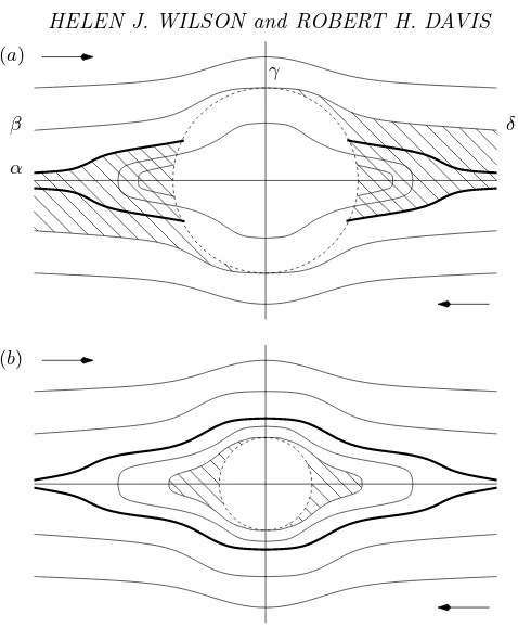
Figure 5. Trajectories in the (x, y) plane of the centre of particle 2 relative to particle 1 in
shear flow, (a) when all closed orbits pass within the contact surface, and (b) when some closed orbits are entirely outside the contact surface. The bold trajectory represents symbolically the trajectory dividing closed orbits from open trajectories. The dotted circles represent the contact surfaces =sc ≡2 +ζ. The shaded region represents forbidden areas where there will be no particles once the flow is well-established; and on the edge of this region there may be a high density of particles.
(I−nn)·E·n= 12γ˙
sinθcosφ(1−2 cos
2θ) cosθ(1−2 sin2θcos2φ)
−2 sin2θcosθsinφcosφ
. (4.9)
In the absence of surface irregularities, there are two types of relative trajectories:
• Open trajectories which arrive from infinity and depart to infinity
• Closed trajectories or cycles. These form the symmetric region
s2sin2θcos2φ < φ2(s)Ψ(s). (4.10) The pair density function is not known for the closed orbits, and so theO(c2) viscosity correction is indeterminate (Batchelor & Green 1972a).
When the surfaces of the spheres exhibit surface irregularities, however, the pattern of relative trajectories is more complicated. Typical surface asperities have height around 10−3–10−2of a particle radius (Smart & Leighton 1989). For two spheres interacting in the (x,y)-plane, this size is large enough that all the closed orbitsin that plane will be affected by contact, and so their symmetry will be broken and the indeterminacy they cause is abolished. This scenario is illustrated in figure 5(a).
pass outside it. This case is shown in figure 5(b). It is important to note that both of these streamline patterns can occur simultaneously in the same flow. Indeed, for any roughness height large enough to break some closed trajectories, there will be both patterns in the same flow, as there are closed orbits whose distance of closest approach is arbitrarily large. This means that the viscosity is always undetermined (as discussed in§4.2).
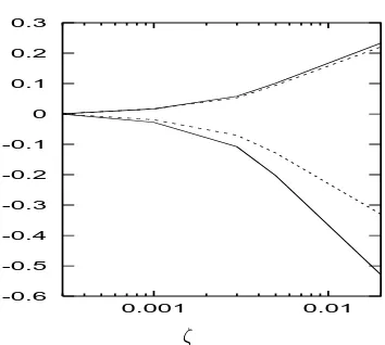
If the height of the surface asperities is very small (i.e. the particles are exceptionally smooth), it is possible for all of the contact surface to fall within the region of closed trajectories. This case occurs when the minimum distance of approach of the trajec-tory dividing closed orbits from open trajectories is greater than the roughness height. Mathematically, it requires that
φ2(sc)Ψ(sc)> s2c, (4.11)
and we have determined (using a numerical interpolation) that this inequality is satisfied whenζ <2.110×10⁻⁴. This roughness height is much smaller than typically encountered, and so it is reasonable to expect that there will be some open trajectories which intersect the contact surface. In this case, as discussed by Rampall, Smart & Leighton (1997), the probability distribution may be calculated in the plane of shear, and so the viscosity of a monolayer suspension of spheres may be calculated exactly. However, if the roughness height is smaller than the distance of closest approach (ζ < 2.110×10⁻⁴), then the surface roughness has no effect, the analysis of Batchelor & Green (1972a) is still valid, and the normal stress differences are zero.
4.2. Calculation of the pair-distribution function
In order to calculate the probability distributionpin simple shear flow, we must consider the following regions of the flow:
• the bulk of the flow: trajectories which originate at infinity and either reach the contact surface or depart to infinity without ever intersecting the contact surface
• closed orbits which do not intersect the contact surface
• the shadow region in which no particles can be found because of contacts which exert compressive but not tensile forces; herep(r) = 0
• the rolling region of the contact surface
• the slipping region of the contact surface
• the border of the shadow region.
The first two of these regions correspond to region (i) of §2.2; the probability density there is unaffected by particle friction.
Unfortunately, the probability distribution is not known on the closed orbits. This fact prevents us, as it prevented Batchelor & Green (1972a) and Zinchenko (1984), from calculating exact viscosity values in this flow unless some distribution is assumed at a given instant in time. To demonstrate the problem of undetermined probabilities in the closed-orbit region, we have chosen two plausible distributions for smooth spheres. In the first case, we take the probability distribution to bep(r) =q(s) everywhere, a distribution which is continuous at the edge of the region of closed orbits. As shown by Batchelor & Green (1972a), the c2 viscosity coefficient in this case isk = 2.5 + 7.5R J qs2ds ≈6.9. In the second case, we assume that the region of closed orbits is well-stirred initially, so thatp= 1 inside this region. As time passes, the probability distribution within the region of closed orbits will fluctuate, but effectively it will oscillate about this value. Therefore it is reasonable to consider a distribution in the outer region which has settled down to its long-term value ofp=q, while the closed-orbit region instantaneously has
18 HELEN J. WILSON and ROBERT H. DAVIS
due to roughness obtained for extensional flow, we cannot hope to deduce definitive information about the effect of surface roughness on the shear viscosity by performing further calculations. Indeed, these calculations would entail a considerable amount of work for conclusions which would be uncertain at the very best.
However, as we shall see, the normal stressesN1= Σ11−Σ22 andN2= Σ22−Σ33 are unaffected by the probability distribution on the closed orbits. We may calculate them without making any further assumptions.
4.2.1. Bulk region
In the first region described above, the fact that the particles are not smooth has no effect on the flow, and the particle trajectories are coming from infinity, and so (2.21) applies. The velocity in the first region is given by (2.7), and so the flux of pairs from this region onto the contact surface is given by
q(sc)Vr(sc) =aq(sc)sc(1−A(sc))(n·E·n). (4.12)
In the region of closed orbits, however, the argument used by Batchelor & Green (1972a) can only give us
p(r) =C(ξ2, ξ3)q(s), (4.13) where ξ2,ξ3 are the invariants of (4.3), and no information is available about the form of C(ξ2, ξ3) unless other effects (such as Brownian motion or longer range forces) are included.
4.2.2. Contact surface
On the rolling portion of the contact surface, the relative velocity of the two spheres is given by (2.13), and that for slipping is given by (2.17). The boundary between rolling and slipping is the point at which the velocity is the same by either mechanism (2.19):
(1−B∗−β4)|(I−nn)·E·n|=−νβ6(n·E·n), (4.14) which turns out, for realistic values ofν (ν ≤0.5, say), to encompass a very small region of the contact surface. Most of the contact surface, therefore, is a slipping region. In particular, the boundary conditionPc = 0 on the edge of the forbidden region must be
applied to the edge of the slipping region.
Unfortunately, the form of |(I−nn)·E·n|, when expressed in terms of the angles θ
andφ, is sufficiently complicated that the partial differential equation which results from the Liouville equation in this case cannot be solved analytically. In turn, the boundary conditions for the rolling region are not known analytically, so that region must also be investigated numerically.
Here, we give the pair of equations which must be solved numerically. To construct them, first we substituteE,Ωandninto the forms ofV (2.13, 2.17). We express all the quantities in trigonometric terms and useX = sinφandY = sinθ, substituting into the Liouville equation
∇·[PcV] =−asγφ˙ −3(sc) sinθcosθcosφ, (4.15) to obtain
∂ ∂X(P
cX[1−α(X, Y)])− ∂ ∂Y(P
cY[1−(1−2Y2)α(X, Y)]) =−4aφ−3(sc)Y2, (4.16)
in which
α(X, Y) =
β4 for rolling
1−B∗−νβ6Y /|f(X, Y)| for slipping
and
f2(X, Y) =[(1−2Y
2)2+X2Y2(3−4Y2)]
4(1−X2)(1−Y2) . (4.18)
This equation is solved numerically in the region
{0≤X ≤1; 0≤Y ≤1} ∩ {Y2(1−X2)> φ2(sc)Ψ(sc)/s2c}
using the method of characteristics, with boundary conditionPc= 0 on the edge of the forbidden region, whereY2(1−X2) =φ2(sc)Ψ(sc)/s2c. The solution can be extrapolated to the rest of the contact surface using symmetry considerations.
4.2.3. Border of the shadow region
The border of the shadow region may consist of
• closed orbits, on which we cannot determine the probability density withoutad hoc assumptions (figure 5b), and
• two surfaces in the wake of sphere 1, of finite extent in they andz directions, and semi-infinite in thex-direction (figure 5a).
We consider only the case when the latter two surfaces exist (though there will also be closed orbits), since the results when there are only closed orbits are exactly the same as for smooth spheres.
In a similar manner to that used in§3, we note that, since there is no flux of probability onto or off the sheet, the Liouville equation is equivalent to mass conservation on the sheet. We parametrise the sheet using the trajectory length, l, and the azimuthal angle at the point of detachment, ˜φ. We also define a quantity dhto be the length element on the sheet perpendicular to the velocity.
We consider a narrow band of trajectories leaving the sphere, and integrate the Liou-ville equation (3.4), with velocity (2.7) over the section of the surface they pass through between leaving the sphere and having travelled a dimensionless distancel. We apply the divergence theorem, noting that the contribution from edges parallel toV is zero, and usingn=V/|V|on the remaining edges and the upstream boundary conditions,
Psh|V|dS =12a2P0shs3c(2−B∗) ˙γ|cos ˜φd ˜φ|dl. (4.19) Now, since dl is the length element parallel to V, we have dl/dt = |V| and of course
ads/dt=Vs. Now|Vs|=|V·n|= ˙γ(1−A)|xy|/as, so
PshdS=P sh
0 a4s3c(2−B∗)s|cos ˜φd ˜φds|
2(1−A)|xy| . (4.20)
Now the valueP0sh is equal to the value ofPc(which is calculated numerically) atθ=π/2. Because the upstream boundary condition is only known numerically, this equation, like that in§4.2.2, may only be used in numerical calculations. However, once the probability has been calculated on the contact surface,Psh
0 is known and therefore PshdS may be found without further integration.
We need information about the shape of the sheet in order to expressx and y as a function ofs and ˜φ. We use the form of the trajectories (4.3), and, applying the initial conditionx= 0, y=ascos ˜φats=sc to determineξ2 andξ3, we obtain
x2
a2s2 = 1−
φ2(s)
φ2(sc)
s2c s2+
φ2(s)
s2 [Ψ(sc)−Ψ(s)], (4.21)
y2
a2s2 =
φ2(s)
φ2(s
c) s2
c s2cos
2φ˜−φ2(s)
20 HELEN J. WILSON and ROBERT H. DAVIS 4.3. Calculation of the normal stresses
Using (2.5–2.6) and (4.2) we can show that the normal stressesN1= Σ11−Σ22,N2 = Σ22−Σ33 will be given by
N1= 15c2µγ˙
4π
Z
r≥2a
n1n2(n21−n 2
2)M(s)p(r) dr
a3
+9c 2µγ˙ 32π
Z
contact
β5
(Fc·n) µγπa˙ 2(n
2 1−n
2 2)−
Fc
1n1−F2cn2
µγπa˙ 2
p(r)dr
a3 +O(c
3), (4.23)
N2= 15c2µγ˙
4π
Z
r≥2a
n1n2[L(s) + (n22−n 2
3)M(s)]p(r) dr
a3
+9c 2µγ˙ 32π
Z
contact
β5
(Fc·n) µγπa˙ 2(n
2 2−n
2 3)−
(Fc
2n2−F3cn3)
µγπa˙ 2
p(r)dr
a3 +O(c
3), (4.24)
and the contribution to the integrals from eis zero. We express the sub-terms of these expressions as
Ni =
15c2µ|γ˙| 4π
ˆ
Nbulki + ˆNcontacti,S + ˆNsheeti
+9c 2µ|γ˙| 32π
ˆ
Ncontacti,D +O(c3), (4.25) wherei= 1 or 2.
4.3.1. Bulk region
In the bulk,F =0since the particles are not in contact, and the contributions to the normal stresses are thus
ˆ
Nbulk1 =
Z
r≥2a
n1n2(n21−n 2
2)M(s)p(r)ds, (4.26)
ˆ
Nbulk2 =
Z
r≥2a
n1n2{L(s) + (n22−n 2
3)M(s)}p(r)ds. (4.27) Throughout the bulk, we have
p(r) =C(ξ2, ξ3)q(s), (4.28) in which C ≡ 1 except on closed orbits. Now s is an even function of n1, whereas the integrand in each case is an odd function ofn1. Thus the contribution from any trajectory along whichn1 is symmetrically positive and negative must be zero. This case includes any closed orbits and also the unbounded trajectories which do not intersect the contact surface.
The only nonzero contribution is therefore from the region of trajectories entering from infinity and intersecting the contact surface. Because they are coming from infinity, these trajectories satisfy (2.21). This region can be expressed as
{xy <0}∩
y2+z2≤a2φ2(s)
s2
c φ2(s
c)
−Ψ(sc) + Ψ(s)
∩{y2≥a2φ2(s)Ψ(s)}, (4.29)
which becomes
{sinθcosθcosφ <0} ∩
sin2θ≤φ
2(s)
s2
s2
c
φ2(sc)−Ψ(sc) + Ψ(s)
∩ {sin2θcos2φ≥ φ
2(s)
This region only exists if Ψ(sc)φ2(sc)≤ s2c, i.e. if there is an intersection between the
contact surface and the open trajectories. As discussed in§4.1, this case corresponds to the reasonable constraintζ >2×10⁻⁴.
Performing the integral overφfirst and then overθ, the first integral (4.26) becomes
ˆ
Nbulk1 = −4 3φ3(sc)(s
2
c−φ
2(s
c)Ψ(sc))3/2×
Z ∞
sc
M(s) (1−A(s))s3
s2+φ2(s)
−s2
c
φ2(sc)−2Ψ(s) + Ψ(sc)
ds, (4.31)
and the second integral (4.27)
ˆ
Nbulk2 = −4 15φ3(sc)(s
2
c−φ
2(s
c)Ψ(sc))3/2×
Z ∞
sc
M(s)φ2(s) (1−A(s))s3
s2
c
φ2(sc)+ 5Ψ(s)−Ψ(sc)
+ 5L(s)
s(1−A(s))
ds. (4.32)
4.3.2. Contact surface
In the contact region we have calculatedPc numerically, and so the total stress
con-tributions ˆNcontacti,S and ˆNcontacti,D must also be calculated numerically. As for strain, we convert the volume integrals to surface integrals using Pc = apds. We substitute
(4.8) and (4.9) into (2.14) and (2.18) for the force dipole. Substituting the definition dS=a2s2
csinθdθdφand using the variables we introduced for calculating the
probabil-ity,X = sinφ, Y = sinθ, we obtain
ˆ
Ncontact1,S =−2M∗s2c
Z 1
−1
Z 1
0
Y2(1−2Y2+Y2X2)P
c
a dYdX, (4.33)
ˆ
Ncontact2,S =−2s2c
Z 1
−1
Z 1
0
Y2(L∗+Y2(1−2X2)M∗)P
c
a dYdX, (4.34)
ˆ
Nroll1,D= 2β2β5
πβ1
s2c
Z 1
−1
Z 1
0
Y2(1−2Y2+Y2X2)P
c
a dYdX, (4.35)
ˆ
Nroll2,D =β2β5
πβ1
s2c
Z 1
−1
Z 1
0
Y2(2Y2(1−2X2)−1)P
c
a dY dX, (4.36)
ˆ
Nslip1,D=+2(1−A ∗)β
5
πβ3
s3cν
Z 1
−1
Z 1
0
Y3
f(X, Y)(1−2Y
2+Y2X2)Pc
a dY dX, (4.37)
ˆ
Nslip2,D=+(1−A ∗)β
5
πβ3
s3cν
Z 1
−1
Z 1
0
Y3
f(X, Y)(2Y
2(1−2X2)−1)Pc
a dYdX, (4.38)
withf(X, Y) as defined in (4.18), so that
f2(X, Y) = |(I−nn)·E·n| 2
˙
γ2(1−X2)(1−Y2). (4.39)
4.3.3. Border of the shadow region