CENTRE FOR ADV
ANCED
S
P
A
TIAL ANAL
YSIS
W
orking Paper Series
Paper 20
HOW
LAND-USE-T R A N S P O R LAND-USE-TALAND-USE-TION
M O D E L S W O R K
Centre for Advanced Spatial Analysis
University College London
1-19 Torrington Place
Gower Street
London WC1E 6BT
Tel: +44 (0) 20 7679 1782
Fax: +44 (0) 20 7813 2843
Email: [email protected]
http://www.casa.ucl.ac.uk
http://www.casa.ucl.ac.uk/working_papers.htm
Date: April 2000 (edited for style November 2000)
ISSN: 1467-1298
ABSTRACT...6
1 INTRODUCTION...6
2 WHY LAND-USE–TRANSPORTATION MODELS?...7
2.1 JUSTIFYING URBAN SIMULATION...7
2.2 THE EMERGENCE OF URBAN MODELLING...8
3 MODEL CLASSIFICATION...9
3.1 BASIC MODELS...9
3.2 MATHEMATICAL MODELS...10
3.3 LAND-USE–TRANSPORTATION MODELS...11
4 DESCRIPTIVE AND ANALYTICAL URBAN MODELS...11
4.1 THE VON THUNEN MODEL...11
4.2 CONCENTRIC ZONE THEORY...13
4.3 WEDGE OR RADIAL SECTOR THEORY...14
4.4 MULTIPLE-NUCLEI THEORY...15
5 GENERAL STRUCTURE OF THE LAND-USE–TRANSPORTATION MODEL...16
6 MODELLING TECHNIQUES...17
6.1 SPATIAL INTERACTION MODELS...18
6.1.1 Production constraints...21
6.1.2 Attraction constraints...22
6.1.3 Production-attraction constraints...23
6.1.4 Entropy-maximizing models...24
6.2 SPATIAL CHOICE MODELS...28
6.2.1 Discrete choice models...28
6.2.2 Non-hierarchical logit models...30
6.2.3 Nested logit models...31
7 INDIVIDUAL MODEL COMPONENTS (SUB-MODELS)...34
7.1 THE LAND USE SYSTEM...35
7.1.1 Location...35
7.1.2 The land development process...41
7.1.3 Supply, demand, and equilibrium...43
7.2 THE TRANSPORT SYSTEM...45
7.2.1 Potential demand modelling and trip generation...46
7.2.2 Trip distribution...47
7.2.3 Modal split...48
7.2.4 Trip assignment (route choice)...48
7.2.5 Accessibility...49
7.2.6 Generalized costs of travel...53
7.3 INTEGRATING LAND USE AND TRANSPORTATION...54
7.4 SIMULATING PLANNING AND PUBLIC POLICY...55
8 THE FAILURES OF LAND-USE–TRANSPORTATION MODELS...56
8.1 THE UNDOING OF URBAN MODELING...56
9 IN DEFENSE OF URBAN MODELLING...57
9.1 URBAN MODELS WEATHER THE STORM...57
9.2 ADVANCING URBAN MODELLING...59
9.2.1 Dynamics...59
9.2.2 Detail...60
9.2.3 Interfacing with the user...60
9.2.4 Flexibility...60
9.2.5 Behavioural realism...61
9.2.6 Zonal geography...61
10 CONCLUSIONS...62
10.2 ENGAGING THE USER THROUGH VISUALIZATION AND APPLICATION...65
10.3 CONCLUSIONS...66
ABSTRACT
This working paper serves as an introductory reference for those studying the application of land-use–transportation models to the simulation of urban systems. The paper is by no means comprehensive, but aims to provide the reader with a foundation in the basic principles underlying land-use–transportation models and to set those principles in the context of urban management and urban studies. The paper opens with taxonomy of urban simulation models and a treatment of descriptive and analytical models. This serves to situate land-use–transportation models in the context of a broader simulation environment. The paper then reviews land-use–transportation models according to their simulation techniques and individual components. Towards the second half of the paper, the discussion moves to a critical overview of urban simulation and deals with model weaknesses and strengths in a holistic fashion, before concluding with a discussion of some innovations in academic research that are likely to shape future models.
1 INTRODUCTION
Computer simulation models combine theory, data, and algorithms to arrive at an abstract
representation of the character and functioning of the land-use–transportation system. Ideally, once
a simulation has been calibrated against a known scenario, the model may be used to make
predictions about the future state of that system. Land-use–transportation models are a particular
class of model used to simulate how land-use and transportation systems operate. They were first
put to use in the management of urban systems to facilitate long-range planning, to simulate the
potential outcomes of decisions affecting the cities, and as a laboratory for testing ideas and
hypotheses relating to urban systems. Since their inception, they have steadily grown in
sophistication and their use has become widespread. However, land-use–transportation models are
uncertain tools—as with any model there is a degree of abstraction in their representation of
real-world systems and processes. Urban simulation is also a relatively unique modelling problem. The
urban systems commonly represented in urban models—economic, social, and environmental—are
notoriously difficult to simulate. Land-use–transportation models are often used to support
decisions that have profound influences upon people’s lives. Also, policies and ideas about the city
are often difficult to experiment with. Equally, the pace of change in urban areas is often such that
models have a hard time keeping up with the phenomena they are simulating.
In the past, researchers and model developers were restricted by their theoretical knowledge about
the city and how it might be simulated as well as being constrained by technological limitations.
Nevertheless, the simulation environment is now appropriate for the infusion of new ideas into
urban modelling. This paper is intended to serve as an introduction to land-use–transportation
as a reference resource.1 The paper deals largely with the techniques that are most prevalent in
operational land-use–transportation models, simply because those ideas form an important
foundation on which to advance urban modelling. Some new emerging techniques in academic
research are introduced, however.
The paper proceeds in Section 2 with a brief overview of modelling and a treatment of the
introduction of models in planning. Taxonomy of models is then developed in Section 3, setting
land-use–transportation models in the context of a broader simulation environment. Some important
descriptive and analytical urban models are mentioned in Section 4, followed by an introduction to
the general structure of the land-use–transportation model in Section 5. Some key modelling
techniques are described in detail in Section 6, providing the reader with a foundation in the
simulation methods that will feature in subsequent sections. Individual model components are then
discussed in Section 7, beginning with the land-use system, and followed by the transport system
and integrated methods for representing the two. In Section 8 the paper moves into a discussion of
the relative merits and shortcomings of land-use–transportation modelling and concludes in Section
9 with a consideration of the future of urban simulations.
2 WHY LAND-USE–TRANSPORTATION MODELS?
2.1 JUSTIFYING URBAN SIMULATION
There are some powerful rationales for applying simulation models to the study and management of
urban systems. In Europe, concerns about the sustainability of our cities is driving a concerted effort
to model their functioning in a bid to forecast future urban patterns. Meanwhile, in the United States
there exists legislation that both directly and indirectly encourages the development of simulation
models of various urban phenomena. This legislation includes the Clear Air Act Amendments:
1
CAAA (1990), the Intermodal Surface Transportation Efficiency Act: ISTEA (1991), and ISTEA’s
successor, the Transportation Equity Act for the Twenty First Century: TEA-21 (1997).
CAAA, ISTEA, and TEA-21 incorporate legislative provisions that mandate land-use–
transportation modelling mostly in its capacity to serve as decision support systems for policies
designed to mitigate urban air problems. However, other initiatives—such as the Travel Model
Improvement Program: TMIP (1992), which was established by the Federal Highway
Administration; the Federal Transit Administration; the Office of the Secretary, U.S. Department of
Transportation; and the U.S. Environmental Protection Agency—have been introduced specifically
to encourage improvements in land-use–transportation modelling.
Other justifications for urban simulation models include the functionality that they offer by
allowing us to test theories and practices about urban systems in a controlled computer
environment. Proceeding from a simulation model, we can evaluate the merits of theories relating to
urban phenomena and test the application of policy measures (such as growth management,
congestion pricing, and pollution mitigation schemes) to various scenarios for urban futures.
2.2 THE EMERGENCE OF URBAN MODELLING
Before proceeding with a discussion of the mechanics of land-use–transportation models, it is
perhaps useful to begin with a review of their history and the academic and social environments that
spawned their introduction into urban planning.
Modelling first became widely applied to urban planning at the beginning of the 1960s. Its adoption
coincided with a general transformation of the character of planning as one identified as
architecture-writ-large to one rooted less intuitively but grounded more objectively (Batty, 1994). In
short, urban modelling emerged as part of an effort to better quantify and mathematically represent
the conditions upon which decisions were made. To facilitate this, model developers, began to
poach analytical methodologies from other disciplines—human ecology, mathematics, geography,
operations research, linear programming, regional science, and economics—modellers were
relentless in their pilfering of scientific techniques that might be applied to urban phenomena. There
were a number of motivating forces driving these changes.
The 1960s was a time of insecurity about the intellectual credentials of urban studies (including
disciplines were quantifying heavily over this period, modelling was, in a sense, a bandwagon
which urban studies researchers felt compelled to jump on in a bid to legitimize the scholarly merits
of their academic pursuits and professional activities.
Underlying and supporting this motivation was a sense of “technological optimism” (Klosterman
1994). Urban models were first used in a period in which it was felt that the scientific successes of
the time (telecommunications, medicine, agriculture, physics, chemistry, and, of course, computers)
could be applied as efficiently and, it was hoped, as successfully to the social realm.
At full swing in their popularity by the early-1960s, urban models were being developed for several
cities in the United States. Large-scale modelling projects were funded in Pittsburgh, San Francisco,
the Penn-Jersey corridor, and elsewhere. Models were also developed for several European cities.
At first they were introduced with the aim of solving land-use and transportation questions, later
being employed with the goal of addressing a wider range of urban problems.
3 MODEL CLASSIFICATION
3.1 BASIC MODELS
Of course, urban models come in many flavours. These range in variety from basic to mathematical
in character, with a respective diversity of theoretical foundations, purposes, and functionality of
use. Nevertheless, a general taxonomy of urban models is presented here as a framework within
which the reader can situate land-use–transportation models. Basic models rarely contain the
capacity for prediction. They may be classified into three main groups: scale, analogue, and
conceptual.
Also known as iconic, scale models are amongst the most well known models. Broadly speaking,
they are scaled-down versions of reality, usually without any functional or predictive capacity.
Essentially, they differ from reality only in size. Examples include wooden block models and
architectural mock-ups.
In analogue models, size is transformed, but so are some of the properties of the thing that is
actually being modelled. The most familiar analogue model, in a geographic sense, is the map. Here
size is reduced (as with the scale model), but so also are some of the properties of the thing being
modelled. For example, in a map scale is reduced, but features are also symbolized (Thomas and
A conceptual model generally expresses how we think a system works. Usually, conceptual models
are presented as arrows that illustrate links or relationships, and boxes representing system
components.
3.2 MATHEMATICAL MODELS
Mathematical models take the ideas encapsulated in a conceptual model and transform them into
mathematical symbology, enabling conceptual ideas to be tested (and in some cases, permitting
predictions to be made). The validity of mathematical models can then be evaluated by comparing
their predictions against observed data. Under the heading of mathematical models there exist a
myriad of sub-classifications, with a variety of goals and techniques. At the broadest level, we can
consider mathematical models to be either normative or deterministic in their goals.
Normative models proceed with assumptions about how a system ought to behave. Deterministic
models, on the other hand, proceed on the assumption that natural, physical laws control the
behaviour of the system being simulated; and that once these laws have been uncovered, the
behaviour of the system can be predicted. As with predictive models, deterministic models are
loosely based on a set of behavioural relationships. Their application to the land-use–transportation
problem is usually concerned with accounting for changes in the spatial pattern of land-use and
transportation systems. They may also be employed to predict or assess the impacts of changes in
exogenous variables or in policies targeted at those systems (Government of Ireland, 1995). Two
important sub-classes of predictive model are probabilistic and optimzing models.
Probabilistic models are deterministic in their assumptions, but are distinct from the broad class of
predictive models in that they express the initial assumptions of the model as a set of probabilities.
In this sense they infuse an element of chance into the simulation process, so that predictions made
by probability models are stated with a known degree of error or tolerance. In this way, probabilistic
models focus on a range of possible outcomes rather than single predictions (Thomas and Huggett,
1980).
Optimizing models apply optimization theory to urban simulation—they assume that the
distribution of urban activities can be allocated so as to optimize some objective function (e.g., the
cost of transportation). The models generally have constraints placed on them to ensure that the
3.3 LAND-USE–TRANSPORTATION MODELS
Land-use–transportation models belong to the mathematical family of models. They are composed
of independent land-use and travel models, with mechanisms for coupling the two—either loosely
or in a more integrated fashion.
Land-use models are used to predict demographic and economic measures of land-based activities.
These measures describe the population (usually in terms of income and employment) and
built-space environment (e.g., floor built-space) for a given urban area.
Travel models (specifically, travel demand models) are used to predict travel patterns on a
transportation network. This class of models aim to simulate travel patterns as a function of human
activities (commonly considered in terms of land uses) as well as the characteristics of the transport
network (commonly considered in terms of accessibility)(Miller et al., 1998).
Integrated land-use–transportation models are used to simulate the interaction of the land use
system and the transport system. Generally, this interaction is simulated by means of feedback
mechanisms. The nature of this interaction will be explored further in later sections.
4 DESCRIPTIVE AND ANALYTICAL URBAN MODELS
Much of the contemporary land-use–transportation modelling effort has proceeded on a foundation
of descriptive or analytical models that have been steadily developed since the beginning of the
Twentieth Century. Among the more influential of these have been the von Thunen model,
concentric zone theory, wedge or radial sector theory, and multiple-nuclei theory. While many of
these models are weak in their theoretical justifications, outmoded in their capacity to describe
today’s cities, and limited in their predictive powers; they have provided both an important
environment for urban simulation and a base upon which contemporary efforts can be built. The
important differentiating factor between descriptive or analytical models and land-use–
transportation models is that descriptive or analytical models offer explanations as to how various
urban phenomena emerge, but they generally abstract from questions of why those patterns
materialize.
4.1 THE VON THUNEN MODEL
Based on a series of simplifying assumptions, von Thunen described a model that would account for
rent-generating capacities dependent upon transportation costs and distance from a central site. Von
Thunen’s model was highly generalized and was based on a series of simplifying assumptions
(Krugman, 1996):
1. The space in which the model was framed was assumed to be an infinite or boundless, flat,
and featureless plane, over which climatic conditions and natural resources were uniformly
distributed
2. The central attracting area was assumed to be a central market
3. Transportation to this central market was assumed to be by horse and cart
4. An allowance for the production and sale of different goods was made, but these goods were
regarded as differing in bulk, therefore having varying costs of transportation from point of
production to the central market
5. For each of these products, transport costs were assumed to vary with distance from the point
of production to the point of sale at the central market
6. The profits to be gleaned from the cultivation of one hectare of land were assumed to be the
same for each product
Based on these assumptions, and operating over the hypothetical space that von Thunen proposed,
he argued that agricultural land uses would segregate into a spatially hierarchic structure akin to that
demonstrated in Figure 1. (As we will see later, the idea is not at all different from bid-rent theory,
Figure 1. The spatial organization of agricultural land uses proposed by the von Thunen model.
4.2 CONCENTRIC ZONE THEORY
EW Burgess developed the concentric zone theory of urban land use in the mid-1920s based on an
examination of the historical development of Chicago through the 1890s. It contrasts from the von
Thunen approach in being descriptive rather than analytical (Harvey, 1996). The concentric zone
theory of urban land use is based on the assumption that a city grows by expanding outwards from a
central area, radially, in concentric rings of development.
Burgess classified the city into five broad zones (Figure 2):
1. The central business district (CBD): the focus for urban activity and the confluence of the
city’s transportation infrastructures
2. The zone of transition: generally a manufacturing district with some residential dwellings
3. The zone of factories and working men’s homes: this zone was characterized by a
predominantly working class population living in older houses and areas that were generally
lacking in amenities
4. The residential zone: this band comprised newer and more spacious housing for the middle
5. The outer commuter zone: this land use ring was dominated by better quality housing for
upper class residents and boasted an environment of higher amenity
Figure 2.The Burgess model of Chicago (after EW Burgess, 1925; Carter, 1981).
While useful in a descriptive sense for explaining the location of land uses in a monocentric city,
both the work of Burgess and von Thunen has (by extrapolation to urban cases), not surprisingly,
come under heavy criticism. Amongst the complaints levelled have been accusations that the
models are too rigid to ever accurately represent actual land patterns (the monocentric city
assumption is perhaps the largest flaw). They have also been accused of overlooking the important
influence of topography and transport systems on urban spatial structure and have been criticized
for failing to accommodate the notion of special accessibility and ignoring the dynamic nature of
the urban land use pattern (Harvey, 1996).
4.3 WEDGE OR RADIAL SECTOR THEORY
Development of the wedge or radial sector theory of urban land use is generally attributed to the
work of Hoyt (1939). Hoyt’s model concerns itself primarily with the location of residential uses
explain the tendency for various socio-economic groups to segregate in terms of their residential
location decisions. In appearance, Hoyt’s model owes a great deal to Burgess’s concentric zone
model: Hoyt presents wedge-like sectors of dominant urban land use, within which he identifies
concentric zones of differential rent. The model suggests that, over time, high quality housing tends
to expand outward from an urban centre along the fastest travel routes. In this way, Hoyt transforms
Burgess’s concentric zones into radial or sectoral wedges of land use (Figure 3).
Figure 3. Hoyt’s sector model (after H. Hoyt, 1939; Carter, 1981).
The innovative element in Hoyt’s model was in considering direction, as well as distance, as a
factor shaping the spatial distribution of urban activity. Hoyt’s model also goes further than its
predecessors in recognizing that the CBD is not the sole focus of urban activity (Kivell, 1993). One
major criticism, however, is that the model overlooks the location of employment, which itself is
the major determinant of residential location (Harvey, 1996).
4.4 MULTIPLE-NUCLEI THEORY
The work of Harris and Ullmann (1945) in developing a multiple-nuclei theory of urban land use is
amongst the most innovative descriptive or analytical urban models. Their model is based on the
premise that large cities have a spatial structure that is predominantly cellular. This, they explain, is
a consequence of cities’ tendencies to develop as a myriad of nuclei that serve as the focal point for
agglomerative tendencies. Harris and Ullmann propose that around these cellular nuclei, dominant
The novelty in multiple-nuclei theory lies in its acknowledgement of several factors that strongly
influence the spatial distribution of urban activity: factors such as topography, historical influences,
and special accessibility. The theory is also innovative in its recognition of the city as polycentric
(Figure 4). In this sense, it moves closer to explaining why urban spatial patterns emerge.
Our attentions will now switch to land-use–transportation models—a class of predictive
mathematical simulations that take many of the theoretical concepts introduced by descriptive and
analytical models and operationalize them by infusing them with empirical data and testing them in
practice.
Figure 4. Diagram illustrating Harris and Ullman’s multiple nuclei model (after CD Harris and EL
Ullman, 1945; Carter, 1981).
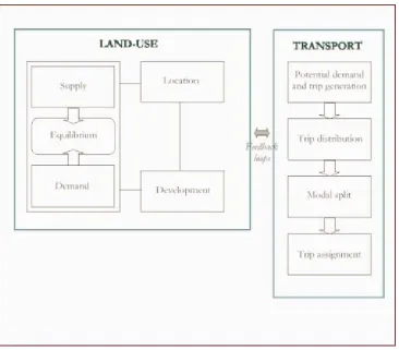
5 GENERAL STRUCTURE OF THE LAND-USE–TRANSPORTATION MODEL
As intuition would suggest, land-use–transportation models couple two distinct systems: land-use
and transport. Embedded beneath the umbrella of these two systems, however, lies an
inter-connected web of sub-models representing various sub-systems and processes at work within the
city. Depending on the peculiarities of the model in question, these sub-models may exist in
isolation from each other, they may be loosely associated, or may be well connected via such
mechanisms as feedback loops.
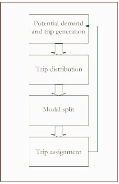
Generally, a number of key components underpinning the land-use–transportation model may be
model to describe transport. The land-use module depends, in varying degrees; on sub-models for
location, land development, and an equilibrium mechanism that balances forces of demand and
supply. The transport system is traditionally simulated via a four-step process beginning with
potential demand modelling and trip generation, proceeding through trip distribution and modal
split, and concluding with trip assignment (Figure 5).
Figure 5. The general structure of a land-use–transportation model.
6 MODELLING TECHNIQUES
The discussion of land-use–transportation models will now proceed with a summary of some of the
key mathematical principles that form the mechanics of most simulations, followed by a detailed
treatment of the various components that comprise the generic model. In Section 6.1 we discuss
spatial interaction models in both their basic and constrained forms. Section 6.2 deals with spatial
6.1 SPATIAL INTERACTION MODELS
The main engine of the generic land-use–transportation model has traditionally been the spatial
interaction model or variants thereof. The spatial interaction model features in land-use–
transportation simulation in its representation of flows of both trips and activities between areas of
the city. While many contemporary simulation packages are moving away from spatial interaction
modelling as a baseline simulation technique, it is worth examining the assumptions and
mathematics underpinning its application to land-use–transportation models, as the technique is still
quite widely used in practice.
A spatial interaction model is generally employed to predict the size and direction of spatial flows
using independent variables that measure some structural property of the spatial area being
modelled. For example, the spatial pattern of journey-to-work flows might be predicted using
structural variables such as the distribution of workers, the distribution of employment, and the
costs of travelling to work.
Based on mathematical assumptions that resemble Newton’s law of gravitational attraction, gravity
models are a particular instance of the broader class of spatial interaction models. Newton asserted
that the force of attraction, F , between two bodies is the product of their masses, m and 1 m ,2
divided by the square of the distance between them, 2
12
d :
2 12 2 1
d m m G
F = ⋅ (i)
where G is a universal constant: the pull of gravity.
Translating this into a geographical context, we could regard force as the number of flows (e.g.,
trips) between two regions and treat mass as a structural variable such as population size. With
these base calculations we can measure a region’s capacity either to generate or to attract trips,
representing distance either in physical terms or in some surrogate form (e.g., travel cost or travel
time).
There are a number of important assumptions underlying the simple gravity model. It is assumed
that the size of any flow is proportional to (∝) a structural variable W at the point of origin for ai
of people, W is often defined as the population of the origin region. Mathematically this isi
represented as:
i
ij W
T ∝ (ii)
which asserts that the magnitude of the flow leaving any region i will grow or decline linearly as the
population size (W ) of the region changes.i
It is also assumed that the size of T (the volume of flows between i and j) is proportional to aij
structural variable W that measures the trip-attraction capacity of the region where the flow ends.j
Again, attractiveness is often measured by the population size of the destination region, or
commonly as the level of employment at the destination:
j
ij W
T ∝ (iii)
which asserts that the magnitude of the flow arriving in any zone j will grow or decline linearly as
the size of opportunities in the destination region change.
Another assumption concerns the measure of distance between the origin region i and destination
region j. It is assumed that the amount of interaction between the two regions, Tij, declines in
proportion with the square of the distance 2
ij
d between the two regions:
2
1
ij ij
d
T ∝ (iv)
or, Tij ∝dij−2 (v)
The validity of this proposition is often justified with data for different types of interaction that
more frequently than long-distance flows do. However, apart from adhering to Newtonian
principles, there is no theoretical justification for expecting flows to decline exactly with the square
of distance between regions. For this reason, it makes more geographical sense to allow distance to
be raised to some power α and to rewrite the assumption more generally as:
α −
∝ ij
ij d
T (vi)
The exact value assigned to α will depend on the available empirical evidence. Raising α to
progressively higher powers steepens the gradient of the curve such that the number of
short-distance interactions is increased relative to the number of long-short-distance interactions. For this
reason the value of α is said to measure the frictional effect of distance.
When the three gravity model assumptions are woven into a cohesive framework, the basic gravity
model formula is obtained:
α
ij j i ij
d W W k
T = ⋅ (vii)
Put simply, this states that flows are a result of push and pull factors. Specifically, that the flow
between two places is a function of the ability of an origin to generate flows (e.g., trips), the
capacity of a destination to attract these flows, the distance over which the flow must pass, and
some weighting mechanism that discourages flows over long distances. In the above equation, the
attraction and generation propositions are incorporated by the multiplication of the terms W andi
j
W . Division by some power of distance produces the distance-decay effect, α. k is a scaling
constant; it needs to be included because the independent variables W and i W are not measured inj
units of flow (Thomas and Huggett, 1980).
Significant variations on this basic description of the gravity model include the
production-constrained model, the attraction-production-constrained model, the production-attraction-production-constrained model,
and the entropy-maximizing model. The motivation behind applying these enhancements to the
model makes. Or, put another way, the notion of the constraint serves as a proxy for the theoretical
notion of market equilibrium. (Although the inclusion of constraints in the gravity model is perhaps
more a function of its weakness in matching observed and predicted flows than of any desire to
reconcile the technique with urban economic theory.) The mechanics of the constrained gravity
model will be explored in detail next.
6.1.1 Production constraints
Essentially, constraints serve to straightjacket a model into reconciliation with known information.
A production constrained gravity model is one in which the total number of flows leaving an origin
i is already known. This knowledge is incorporated into the model design. To recap, let us restate
the original gravity model equation and then examine how that formulation changes with the
application of a production constraint. The basic gravity model may be formulated as follows:
α
ij j i ij
d W W k
T = ⋅ (viii)
The production-constrained model is a confined version of this formula, where the following
constraint is satisfied:
i n
j
ij O
T =
∑
(ix)Here,
∑
n
j
sums the values of O (usually a value for the population size of a trip origin zone)i
across all destinations j; T is the predicted flow between origin i and destination j; and ij O is thei
known total number of flows beginning in origin zone i. What the production constraint secures,
then, is that the sum of all flows predicted as originating in zone i actually conform to the total
urban system in advance of beginning the simulation process, so we can constrain the model to
prevent over- or under-predicting of this figure.
Adding the production constraint to the model yields:
α −
= i i j ij
ij AOW c
T (x)
where T is the predicted flow of trips (or a flow of any commodity in the urban system) betweenij
origin i and destination j, O is the total known number of trips beginning in origin i, i W is thej
attractiveness of destination j for the flow (e.g., floor space or employment), and cij−α is cost of
travel between i and j with a distance decay effect applied. A has replaced k in the basic model.i
Here, A is a scaling constant for each origin i that ensures that the sum of the flows leaving zone ii
for destinations j sum to the known total zonal flow count. In this sense, A is the ratio between thei
known flow from i and the sum of the unscaled predicted flows leaving origin i for destination j.
Mathematically this can be represented as:
∑
−= n
j
ij j i
i i
c W O
O A
α
(xi)
6.1.2 Attraction constraints
In an attraction-constrained model, we know how many trips have reached destinations j in an urban
system. Again, the predicted trip matrix is made to satisfy a constraint, this time in the form:
j n
i
ij D
T =
where D is the known number of trips reaching a destination j (e.g., the number of jobs at aj
destination j, or perhaps the allure of shopping facilities there).
Incorporating the constraint fully into our basic gravity model yields the formula:
α −
= j j i ij
ij B DWc
T (xiii)
where D is the known number of trips reaching destination j, j W is the attractiveness of origin i asi
a residential location, and cij−α is cost of travel between i and j with a distance decay effect applied.
j
B is a scaling constant; for any destination zone j, B is calculated as the ratio between the knownj
number of jobs in that destination (D ) and the sum of the unscaled unpredicted journey-to-workj
flows arriving in destination zone j from each origin zone i (Thomas and Huggett, 1980).
Mathematically, B is derived from:j
∑
−= n
i
ij i j
j j
c W D
D B
α
(xiv)
The attraction constrained gravity model may be considered to be a residential location model in the
sense that it uses knowledge of the distribution of jobs, the residential attractiveness of each zone,
and journey-to-work costs to assign workers to households in the city.
6.1.3 Production-attraction constraints
The singly constrained gravity model (either of the production- or attraction-constrained models in
isolation) essentially becomes a location model. However, if both flow origins and flow destinations
are constrained in the model framework, our attention returns to predicting the size of individual
flows are asked to satisfy two constraints simultaneously (the production and attraction constraints
already discussed):
i n
j
ij O
T =
∑
(xv)and
∑
=n
i
j
ij D
T (xvi)
Incorporating these into the basic gravity formula yields:
α −
= i i j j ij
ij AOB D c
T , (xvii)
with the scaling properties A and i B defined as before.j
6.1.4 Entropy-maximizing models
The notion of entropy offers a theoretical framework for spatial interaction models. Based on
statistical mechanics, entropy is concerned with finding the degree of likelihood of the final state of
a system. Data for urban systems are not usually abundantly available. We therefore need a method
for making reasoned estimates of the likely state of an urban system using the information that we
do know. In this sense, we maximize entropy subject to constraints of known information.
There are two important concepts in entropy that are applied to urban contexts—the macrostate and
the microstate. If we consider our urban system to be comprised of flows between origins and
destinations, we may think of the macrostate description of our system as being the numbers of
individuals or items flowing between origins and destinations. This macrostate is composed of
many microstates—descriptions of the actual individuals or items that make up a macrostate. Just as
there are many possible arrangements of individuals that could make up a subway train of two
hundred commuters travelling from one location to another, there are many possible microstates
The number of microstates associated with any given macrostate can be calculated as:
∏
= n
i i
N N R
! !
(xviii)
where R is the number of microstates associated with any given macrostate for the system, N is
the number of individuals or items assigned to a set of categories, N is the number of individualsi
in a category i , !N is the factorial value of N : )N(N −1)(N −2)(N −3)...(N−n , and
∏
n
i
is the
product of a factorial value.
Framed in this context, the problem of modelling spatial flows then becomes one of maximizing
entropy—choosing the macrostate associated with the largest number of microstates (Barra, 1989;
Fotheringham et al., 2000; Fotheringham and O'Kelly, 1989). If we consider our flows to be trips
from origin i to destination j , we can substitute T (the total number of trips made in our system)
and T (the individual flow of trips from an origin to destination) for N and ij N in the abovei
equation:
∏
= n
ij ij
T T R
! !
(xix)
In dealing with something as complex as an urban system, a modeller can end up with many
possible states to pick from in her or his choice set. As with the basic gravity model, constraints
may be introduced into the entropy-maximizing framework, allowing us to reduce the choice set of
predicted trip matrices down to a manageable level. This constraint is placed on the state description
as:
∑∑
n =i
ij n
j
ijc C
where c is the cost of travel from zone i to zone j, and C is the overall expenditure available forij
those trips.
Once an entropy value has been approximated, it needs to be maximized to arrive at a solution to
our problem of identifying the most likely trip matrix from a potentially infinite number of possible
forms. The maximization of the entropy value is involves the use of Lagrange multipliers (a
technique for evaluating maxima or minima of a function subject to one or more equality
constraints). Essentially, the Lagrange multipliers serve as weightings to ensure that the constraints
within the model are met. Incorporating constraints, the model may be expressed mathematically as:
− + − + − +
=
∑
∑
∑
∑
∑
ijn ij ij n j n j ij j j n i n j ij i
i O T D T C T c
W
L ln τ α β (xxi)
where L is the function to be maximized subject to constraints; τi is the Lagrange multiplier
associated with a production constraint; αj is the multiplier associated with an attraction constraint
(and if both production and attraction constraints are included the model may be considered to be
doubly constrained); and β is the multiplier associated with a cost constraint. The trip matrices that
maximize L , i.e., the most likely distributions of trips in the urban area, are solutions of the
calculation: 0 = ∂ ∂ ij T L (xxii)
To solve this equation we make use of Stirling’s approximation when the values of T are large:ij
x x x
x!= log −
log (xxiii)
ij j i ij ij c T T L β τ τ − − − − = ∂ ∂ ln (xxiv)
Setting the equation to zero and solving yields:
)
exp( i j ij
ij c
T = −τ −τ −β (xxv)
One of the innovative features of the entropy approach to spatial interaction modelling is that it
provides a theoretical (albeit derived from statistical mechanics) for a family of spatial interaction
models. By substituting the above equation in place of T in our constraint models already exploredij
in Section 6.1 we derive entropy versions. For the origin constraint, the equivalent entropy model is
derived as: i n ji ij
O
T
=
∑
becomes1 ) exp( ) exp( − − − =
−
∑
ijn
j
j i
i O τ βc
τ (xxvi)
and for the destination constraint, the equivalent equation is:
j n
i
ij D
T =
∑
becomes1 ) exp( ) exp( − − − =
−
∑
ijn
i
i j
j D τ βc
τ (xxvii)
To see how this results in a full spatial interaction model, we simply add our scaling constants, Ai
and B :j
j i ij j
i
ij OD c AB
This represents the entropy spatial interaction model in its general form. From that equation, four
versions may be derived: origin-constrained, destination-constrained, doubly-constrained, and
unconstrained.
6.2 SPATIAL CHOICE MODELS
6.2.1 Discrete choice models
As has already been mentioned, there is little theoretical justification to support the notion that
urban systems operate in a fashion akin to Newtonian gravity. At the start of the 1970s, some
serious criticisms were levelled against gravity-type formulations of land-use–transportation
models. In reaction to this, modellers began to develop simulations that were more behaviourally
grounded. One avenue of development that was widely embraced was that of discrete choice
modelling. Broadly speaking, discrete choice models (which derive from decision theory) are
concerned with explaining phenomena in terms of decision-making. While they function in a
fashion that resembles spatial interaction models, they are actually concerned with spatial choice.
The most widely used manifestation of the discrete choice model in urban simulation is the random
utility model and variations thereof.
Random utility models proceed on a number of assumptions. The first assumption specifies that
each decision-maker is faced with a discrete set of choice alternatives—a choice is either made or
not made. The second assumes that an individual (or a group of individuals) will settle upon one
decision from a larger set of available options in such a way that the most utility, or satisfaction, is
yielded. Contextualizing this in an urban sense, we might think of a household making a location
decision amongst a set of given locations that a city has to offer so that a combination of utilities is
maximized (e.g., cost, amenities, quality of the school system, etc.). The third assumption in
random utility models is that choices are made in a probabilistic fashion—decision-makers have a
likelihood of making certain choices. Finally, it is assumed that the utility of a decision can be
divided into two components: one measuring ‘strict utility’: the fixed and measurable attributes of
utility, and the other dealing with stochastic utility: an error or disturbance term that reflects the
unobserved attributes of a given decision (Barra, 1989; Golledge and Stimson, 1997).
Mathematically, we can build up a formula for the random utility model based on these
ij
ik U
U > ∀k ≠ j,j =1,,n (xxix)
where U is the utility of a decision-maker i making choice k; ik U is the utility of a decision-makerij
i making choice j; and ∀k ≠ j,j=1,,n asserts that j stands for all choices other than k. Simply then, the above formula establishes a framework for a decision to be chosen from a set of
alternatives.
Introducing the idea of probabilistic decision-making develops the random utility formula further:
[
ik ij]
ik U U
P =Pr > ∀k ≠ j,j =1,,n (xxx)
where P is the probability of a decision-maker i choosing alternative k; and Pr is a probabilisticik
expression. This assigns likelihood to various choices from a set of alternatives.
Adding the assumption that utility may be distilled to a ‘strict utility’ and stochastic component
yields the final random utility model formula:
[
ik ik ij ij]
ik V E V E
P =Pr + > + ∀k ≠ j,j=1,,n (xxxi)
where V and ik V are the ‘strict utility’ components of an individual i’s choices of k and jij
respectively and E and ik E are the stochastic elements of the utility calculation for choices k and j.ij
Additional elements may be added to this formula to weight the probability calculation, e.g.,
variables representing the socio-economic characteristics of a decision maker.
The random utility model has many similarities to the entropy-maximizing gravity model. There are
important differences though. Their similarities may be in large part a function of the set of
assumptions upon which they are formulated, rather than their theoretical justifications or actual
mechanics. There is also a difference in the way the two approaches handle the assumptions under
which they operate, particularly in how they order them. Entropy models assume choices to be
utility models, on the other hand, start out with an assumption of a rational choice base, and
introduce a random element as they proceed (Government of Ireland, 1995).
6.2.2 Non-hierarchical logit models
The most common derivative of the random utility model is the multinomial logit model. The logit
model expresses the decision choice as a function of the utility of choosing one alternative over
another. The model is derived by making assumptions regarding the random component of utility,
ij
E .
A common assumption is that the distribution of E follows a Weibull distribution (also known as aij
double exponential or extreme value type I distribution). The assumption of a Weibull distribution
affords the utility calculation a greater degree of mathematical tractability. Applying the Weibull
function to the random component of utility leads to McFadden’s logit model, in the form:
(
)
[
]
(
)
[
]
∑
= n j i j ij i k ik ik S X V S X V P , exp , exp (xxxii)where X and k X are the choice specific attributes of choices k and j respectively (e.g., in terms ofj
trip-making, this could represent costs, time, etc.); and S is the individual-specific attributes ofi
choice k (e.g., the decision-maker’s income, level of auto ownership, etc.). In short then, the
McFadden logit model states that the probability of a decision-maker choosing an alternative k from
a set of available alternatives is a function of the attributes of the available alternatives and the
decision-maker’s own characteristics (Government of Ireland, 1995).
The non-hierarchical logit formulation suffers from some serious weaknesses however.
Behaviourally, the logit framework assumes that individuals evaluate every available alternative to
their decision before settling on an optimal one. In practice, cities generally offer far too many
competing alternatives to any given decision to be completely evaluated in this manner. Rather,
decision-makers, be they individuals or groups, are more likely to settle on a final decision from a
small subset of the available alternatives that are globally available to them throughout the entire
urban system. A hierarchical decision-making strategy is thus more likely to be employed than an
weaknesses owing to the independence from irrelevant alternatives problem and the assumption of
regularity. The problem of independence from irrelevant alternatives (popularly known in transport
modelling as the ‘red-bus-blue-bus conundrum’) lies in the fact that logit models assume that the
ratio of probabilities of an individual selecting two alternatives is irrelevant from the addition of an
extra alternative. Yet, the introduction of additional alternatives is generally quite relevant in spatial
terms. Closely related to this is the idea of regularity, which refers to the notion that within the logit
framework it is not possible to change the probability of selecting an alternative by adding another
alternative to the choice set (Fotheringham and O'Kelly, 1989). In the context of an urban system
this assumption holds little value; it leaves the decision-making process unaffected by any offer of
additional choices to a decision-maker.
6.2.3 Nested logit models
The nested logit model departs from the basic logit formulation by introducing hierarchy into the
decision-making process. Nested models assume that decision-makers process information about
choices in a chained fashion and that the modeller is aware of the form of that chain. In this sense
they attempt to circumvent the weaknesses of the non-hierarchical model by assuming that decision
makers make choices sequentially, rather than wading through every available option at once.
A common application of the nested model is to travel choice. Various sequential stages in the
decision to travel can be identified, e.g., whether or not to make a trip; where to go; by what mode a
trip should be made; and on what route to travel. This method of simulation abstracts from
irrelevant (or less relevant) information regarding the decision, and focuses the choice on the set of
alternatives that are most applicable. Mathematically, this results in a set of conditional probabilities
for each of the sequential stages in the decision-making process. Aggregating these probabilities
yields the likelihood of a choice being made such that:
(
abcd) ( ) ( ) (
P a P b a P c a b) (
Pd a b c)
P . . . = | | , | , , (xxxiii)
where a, b, c, and d refer to the four sequential stages in the decision hierarchy (e.g., whether to
step in the hierarchy and work its way back to the beginning in order to ensure that the strict utilities
are preserved throughout the process (Government of Ireland, 1995).
Formulating the nested model in spatial terms, decision-makers can be regarded as choosing options
from a set of clusters. Continuing with our making analogy, we now have individual
trip-makers (or perhaps groups of trip-trip-makers) who make decisions about their trips but also have to
consider a range of spatial options in which to focus those choices. Mathematically, this can be
represented as:
( )
( )
( )
( )
∑
∑
∑
= ∈ ∈ n s n s k ik is n s k ik is is V V V V P σ σ exp exp exp exp (xxxiv)where P is the probability that a decision-maker i will select a particular spatial cluster s to focusis
its decision in;
∑
( )
∈ n s k ik V
exp is termed an ‘inclusive value’ and describes the attractiveness of a
cluster as a function of the individual alternatives available within that cluster (Fotheringham and
O'Kelly, 1989); and σ represents the extent to which decision-makers process their information
hierarchically, and ranges in value from zero to one, with σ =1 denoting decision-makers who do
not process their information hierarchically at all.
Once a decision-maker has selected a given spatial cluster, s, to narrow her choice set, all that
remains is for an option (or alternative), k, to be settled upon. The likelihood of a
decision-maker selecting a particular alternative k, within the selected spatial cluster s, is then calculated as:
( )
( )
∑
∈
∈ = n
s k ik ik s ik V V P exp exp
∀k∈s (xxxv)
s ik is
ik P P
P = ∈ (xxxvi)
Spatial choice models are perhaps more appropriate representations of how land-use and
transportation systems organize than spatial interaction models, but they suffer from weaknesses.
Notably, it is widely understood that the distinctions between choice categories may often be fuzzy
rather than discrete. Spatial choice models do not commonly accommodate this.
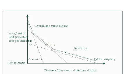
6.3 BID-RENT THEORY
Figure 6. Diagram illustrating land use patterns distributed spatially across a theoretical city
according to bid-rent theory
The final modelling technique, which along with spatial interaction and spatial choice, underlie the
most common land-use–transportation models is bid-rent theory. Bid-rent theory (popularized by
Alonso) owes a great deal to the von Thunen model that we explored in Section 4, as Figure 6
illustrates. Proceeding from a set of simplifying assumptions (notably, monocentric cities and a
limited range of land uses), bid-rent theory offers an explanation of the spatial distribution of urban
activities. The central argument of bid-rent theory is that land uses will organize geographically
value, profit, or utility that an activity places on accessibility to a central urban core. Given these
considerations, land uses will tend towards a spatial arrangement akin to that illustrated in Figure
6—with businesses located close to the urban core and industry and residences situated towards the
urban periphery.
While the notion of bid-rents has enjoyed a wide application in urban modelling, and has a limited
theoretical justification, the theory does not easily transfer to practice. The utility function, in
particular, can be difficult to calculate. Often, it involves a monetary component (e.g., travel time
and/or travel cost related to distance from work). But in many circumstances the utility function
also contains non-monetary conditions that are difficult to cost—the availability of space, fresh air,
peace and quiet; location prestige; neighbours; family ties; etc. (Balchin and Kieve, 1977).
Nevertheless, bid-rent theory enjoys a pivotal position in many operational land-use–transportation
models and is an important ingredient in their formulation.
A variant of bid-rent models—hedonic price models—has gone further towards operationalizing
some of the factors that weigh into the bid-rent calculation. Hedonic price models distil real estate
values into constituent components (e.g., land value, structure value, number of bedrooms in
property, proximity to schools, etc.), each of which has an associated value. Often these models can
be incredibly disaggregated. However, they are weakened to some extent by their reliance on price
as a framework for formulating ideas about the dynamics of urban systems. Also, because of
privacy concerns, price data can be difficult to obtain, especially data spanning multiple time
periods. Moreover, many things are difficult to price.
7 INDIVIDUAL MODEL COMPONENTS (SUB-MODELS)
With a grounding in the important modelling principles common to land-use–transportation models
behind us, the discussion now moves onto a treatment of the various sub-models that make up
land-use–transportation models. In Section 7.1 simulation of the land use system will be described in
terms of location, development, and equilibrium; then the focus will shift in Section 7.2 to a
representation of the transport system, discussed in terms of potential demand modelling and trip
generation, trip distribution, modal split, trip assignment, accessibility, and the generalized costs of
travel. Ways of integrating the land-use and transport systems in a simulation are then mentioned in
7.1 THE LAND USE SYSTEM
The essential components of the land use system, in terms of land-use–transportation modelling, are
location and development.
7.1.1 Location
The urban land use system is largely modelled by simulating the mechanisms that affect the spatial
location of urban activities in a city. The most important of these location factors for simulation
purposes—accessibility—will be discussed in more detail in later sections. A number of other
important geo-economic concepts underpin land-use–transportation models, serving as proxies for
the complex interactions and motivations driving urban location. Among these are the ideas of
bid-rent, travel costs, inertia (stability in the occupation of land), topography, climate, planning, and
size.
As the discussion surrounding bid-rent theory alluded to, not all land uses in the city have the same
location considerations. It is useful, therefore, within a land-use–transportation model, to
decompose the location decision to represent a broad classification of the most important land uses
in a city. Residential location and firm location are essential considerations, and occasionally
industrial location is modelled.
7.1.1.1 Residential location
There are three main theories explaining the rationales underlying urban residential location:
bid-rent theory, travel cost minimization theory, and travel cost and housing cost trade-off theory.
Expressing the household location decisions of two households in a monocentric city in a bid-rent
Figure 7. Diagram illustrating a residential bid-rent curve for a monocentric city.
When seeking out a location (in this conceptual, economic sense), each household pursues a
location on the bid-rent curve where the land price curve touches the bid-rent-curve nearest the
origin, i.e., a household seeks the location that yields the greatest utility at current market rents
(Harvey, 1996). The shape of a household’s bid-rent curve is dependent upon their particular
situation (tastes, income, etc.). For example, a young family (household B) will generally require
space and access to schools. Its bid-rent curve is likely to be relatively flat as a result (implying that
a household is more likely to locate in the suburbs). On the other hand, single people, the elderly, or
families consisting mainly of wage earners (household A), are likely to have steeper bid-rent curves,
and may favour locations closer to the CBD.
Travel cost minimization theory assumes that the only consideration in the residential location
decision is that households select locations that reduce their need to travel. If we consider a city
with jobs located in a central core, this implies that the most sought after locations would be close
to the CBD, while the less popular areas would be concentrated on the urban fringe.
Socio-economically, this would suggest concentrations of wealthy households in the central city, with
poorer households towards the urban periphery. In reality, the cost of travel is not the only
residential location factor affecting the decisions of households; factors such as open space and
quality of housing muddy the issue and the opposite is generally true: the poor end up closer to the
CBD and the rich live farther out. Also, jobs are increasingly located in the suburbs. Nevertheless,
travel cost minimization theory does have some relevance to household location (particularly
Travel cost and housing cost trade-off theory assume that households trade off the competing
influence of housing cost and travel cost in making their residential location decision. This implies,
in geographic terms, that land values will be higher close to a central business district and lower
towards the periphery. While this is largely true in practice, there are many complicating factors,
both economic and non-economic. High-income households may not have to trade off housing cost
against travel cost, because they may be able to afford both. People who can afford to live close to
the CBD may elect not to because they wish to enjoy the amenities on offer in the suburbs (e.g.,
environment, space, and for reasons of segregation). Because of the dearth of available space in
central cities, outer areas generally offer a wider range of opportunities for the construction of new
and expensive houses. Also, transportation innovations may make outer locations more accessible
to a CBD than inner suburban areas. This is significant; jobs are increasingly relocating to
peripheral sites. Additionally, location decisions may be heavily reliant on the availability of
income and mortgage finance, which is often distributed aspatially within a given metropolitan area.
And there may be a time lag before households react to changes in housing costs.
There are also many non-economic reasons that play equally important roles in affecting household
location decisions. For example, some households may have a low degree of mobility in their
decision to move. There may also be more pressing familial reasons why a household seeks to
move, and governing the type of real estate they may demand, e.g., changes in employment,
marriage, family size, and age.
7.1.1.2 Business location
Households may desire central areas as much as other urban land uses, but they can rarely hope to
outbid uses such as industry and business (unless the residences compose multi-storey blocks of
residential units) because they cannot derive as much profit (or utility) as those other uses. In terms
of bid-rent, firms generally out-bid all other activities in the urban location decision, simply because
they can derive the most profit from occupying a particular site. In this sense, they tend to have the
steepest bid-rent curves (Figure 6). We find that firms tend to locate where the land price curve
touches the bid-rent curve. At that point, the most profitable location at current market rents is
realised, which is often in, or close to, the CBD. However, firms requiring large sites may have a
flatter bid-rent curve (firm B), and may locate in suburban areas or towards the urban periphery
(Figure 8).
7.1.1.3 Industrial location
Industrial land uses have the same need for proximity to central sites as do firms. Their location
motivation is also similar to that of firms: availability of labour, access to transportation, auxiliary
services, etc. However, their need for central locations is not as great. As a result, industries are not
as well equipped to compete for central sites and their rent gradients tend to be flatter than those of
commercial firms.
In recent years there have been significant changes in the location behaviour of most urban
land-uses because of advances in the provision of transport infrastructure, changing socio-demographics
amongst urban populations, and alterations in the spatial structure of the city. While these
reorganizations have affected all urban land uses, the impact of these changes has been particularly
profound for manufacturing industry and its location within metropolitan areas. Manufacturing uses
have been persuaded or forced out of central locations largely because of developments in the
provision of roadways—the contemporary wave of road building has focused mainly in outer urban
areas. Nevertheless, a large degree of inertia remains for centrally located manufacturing industry,
fuelled by traditional preferences for downtown sites and the benefits of external economies of
agglomeration in central areas.
7.1.1.4 Simulating location via the Lowry framework
One way of handling the idea of location in a simulation sense is via the Lowry framework.
place of employment governs the place of residence—jobs decide where people live. In the Lowry
framework, employment is divided into basic (mainly manufacturing) and non-basic (mainly
service) sectors. The framework takes basic employment (which must be exogenously supplied)
together with endogenously derived service employment and uses them to estimate the location of
residents. This estimate of residential location is then fed back into the model to predict the location
of service employment. The model then proceeds iteratively through these steps, assigning activities
to urban locations.
Lowry’s assumption that basic industry should be exogenously determined (outside the model) was
based on his observations that basic industry has specialized site requirements and external markets,
and that its location decisions are independent of the residential population (Oryani and Harris,
1996). However, Lowry suggested that service employment be endogenously derived (within the
model) since its location decisions are closely related to residential demand. He also assumed that
the residential location decision was made in relation to both combined service and basic
employment.
Distilling the Lowry framework to its two principal mechanisms—residential and firm location—
presents a clearer idea of how the model operates. In the residential component, population (or
households) are assigned to residential locations in origin zones based on their places of
employment in destination zones. Two main factors are used to govern this location assignment
process: zonal attractiveness and distance. For households, zonal attractiveness can be characterized
by variables such as floor space; housing prices or rents; availability of schools, shops, health
services, leisure and recreation facilities, etc. The other factor—distance between places of
residence and work—may be considered in physical terms or as the cost of traversing that distance
in monetary costs or time expenditure.
In the service employment (firm) component, firm location is directly linked to residential location,
implying that service employment is located either alongside, or soon after, residences. The major
factors driving service employment are governed to be accessibility to consumers and rental costs
for work sites.
The Lowry model is expressed mathematically as a series of singly constrained spatial interaction
models. It proceeds sequentially and iteratively through four main stages. In the first step, basic and
service employment totals are combined and this figure is used to estimate total employment in a
destination zone. (Service employment totals are usually set to zero in the first iteration.)