An Expansion Based on Sine-Gordon Equation to Solve KdV and modified KdV Equations in Conformable Fractional Forms

(1)

An Expansion Based on Sine-Gordon Equation to

Solve KdV and modified KdV Equations in

Conformable Fractional Forms

Ozlem Ersoy Hepson

a

, Alper Korkmaz

b,∗

, Kamyar Hosseini

c

,

Hadi Rezazadeh

d

, Mostafa Eslami

e

a_Eski¸_{sehir Osmangazi University, Department of Computer and Mathematics, Eski¸}_{sehir, Turkey.}

b_C_{¸ ankırı Karatekin University, Department of Mathematics, 18200, C}_{¸ ankırı, Turkey.}

c_{Department of Mathematics, Rasht Branch, Islamic Azad University, Rasht, Iran.}

d_{Faculty of Engineering Technology, Amol University of Special Modern Technologies, Amol, Iran.}

e_{Department of Mathematics, Faculty of Mathematical Sciences, University of Mazandaran, Babolsar, Iran.}

Abstract

An expansion method based on time fractional Sine-Gordon equation is implemented to construct some real and complex valued exact solutions to the Korteweg-de Vries and modified Korteweg-de Vries equation in time fractional forms. Compatible fractional traveling wave transform plays a key role to be able to apply homogeneous balance technique to set the predicted solution. The relation between trigonometric and hyperbolic functions based on fractional Sine-Gordon equation allows to form the exact solutions with multiplication of powers of hyperbolic functions.

Keywords: Sine-Gordon Expansion Method; Conformable time fractional KdV Equation; Conformable time fractional modified KdV Equation; Exact Solution, Traveling Wave Solution.

MSC2010: 35C07;35R11;35Q53.

PACS: 02.30.Jr; 02.70.Wz; 04.20.Jb

∗_{[email protected]}

(2)

1 Introduction

Probably the most famous and fundamental weakly nonlinear PDE with soliton type wave solutions in shallow water surface is Korteweg-de Vries (KdV) equation. Even though it was firstly introduced by Boussinesq [1] in 1877, it is named after the study of Korteweg and de Vries [2]. The KdV equation is completely integrable and has wave solutions of classical solitary wave type shapes. Moreover, it has infinitely many conservation laws representing various physical quantities such as mass, momentum, energy, etc. preserved during motion [3]. The equation can describe many types of physical phenomena particularly waves covering internal ocean waves in changing density layers, plasma ion-acoustic waves and acoustic-type waves over crystal lattice.

The KdV equation is similar to nonlinear Schr¨odinger equation due to the fact that both are solvable by inverse scattering transform approach. It has stable N-soliton solutions that behave like particles, too [4]. These solutions are valid for multiple collisions,i.e. more than two well-separated solitons, even when their heights are different from each other [5].

Recent developments in computer algebra lead various solution techniques to ap-pear. Different forms of tanh −coth method was implemented to the KdV equa-tion to determine periodic and soliton type wave soluequa-tions [6]. (G0/G)-expansion method is also capable of setting the exact solutions of the KdV equation in vari-ous rational forms of hyperbolic or trigonometric function series [7]. Some periodic solitary type wave solutions are determined by extended form of homoclinic test method [8].

The modified form of the KdV (mKdV) equation is obtained by changing the non-linear termuuz tou2uz in the KdV equation. Wronskian expansion technique was

used to determine composite function solutions to the mKdV equation [9]. Imple-mentation of simple sin −cos ansatz techniques gives some traveling type wave solutions in forms of trigonometric and hyperbolic functions [10]. The exp function approach also determines some periodic solutions including the rational functions of exponential and trigonometric function in both numerator and denominator [11]. In this study, we focus on the conformable time fractional forms of the KdV equation

D_tγu+puuz+quzzz = 0, t >0, γ ∈(0,1] (1)

and the modified KdV equation

Dγ_tu+pu2uz+quzzz = 0, t >0, γ ∈(0,1] (2)

(3)

such as various forms of Kudryashov approach, exponential rational function tech-nique, simple hyperbolic ansatzes [13–22], the fractional form of the Sine-Gordon equation method is implemented to both equations to derive exact solutions in traveling wave forms. Before constructing the solutions, some preliminaries and basic properties of conformable derivative are given below. A brief summary of the method is also given in the next sections.

2 Preliminaries of Conformable Derivative

γ.th order conformable derivative of a conformably differentiable functionT =T(t) is defined as

D_tγ(T(t)) = lim

→0

T(t+t1−γ)−T(t)

τ , t >0, γ ∈(0,1]. (3)

where T = T(t) : [0,∞)→ _R [12]. This form of the fractional derivative satisfies many properties required to be able to study to solve non linear fractional PDEs. Some of these properties can be summarized in the following theorem.

Theorem 1 Let S = S(t) and T = T(t) are γ-differentiable in the positive part of t-axis. Then,

• D_tγ(k1S(t) +k2T(t)) =k1Dγt(S(t)) +k2Dtγ(T(t))

• D_tγ(tm_{) =}_mtm−γ_,_∀_m_∈

R

• D_tγ(k3) = 0, for all constant functions S(t) = k3

• D_tγ(S(t)T(t)) = S(t)D_tγ(T(t)) +T(t)Dγ_t(S(t))

• D_tγ(_TS(₍t_t)₎) = T(t)D

γ

t(S(t))−S(t)D γ t(T(t))

T2₍_t₎

• D_tγ(S(t)) =t1−γ dS(t)

dt

for ∀k1, k2, k3 ∈R [23].

This newly introduced fractional derivative satisfies plenty of helpful properties. Some of these properties like the chain rule, some integral transforms, and Taylor series expansion were summarized in [24]. The following theorem gives the relation between the classical and conformable derivative.

Theorem 2 Let S=S(t) be a γ-conformable differentiable function. Then,

D_tγ(S◦T)(t) =t1−γT0(t)S0(T(t)) (4)

(4)

3 Sine-Gordon Equation (SGE) Method

Consider the one dimensional time fractional SGE of the form

∂2_u ∂z2 −D

2γ

t u=c2sinu, c is constant (5)

where u=u(z, t). The fractional traveling wave transform

u(z, t)→U(η)

η=a(z−νtγ/γ) (6)

reduces the time fractional SGE (5) to

d2_U dη2 =

m2

a2₍₁₋_ν2₎sinU (7)

where ν is speed parameter of the wave defined in the fractional traveling wave transform [25]. After some calculus, the equation is reduced to

d(U/2)

dη

2

= m

2

a2₍₁₋_ν2₎sin

2_U/_{2 +}_C ₍₈₎

where C is integration constant and assumed zero. Assume that w(η) = U(η)/2 and m2_/₍_a2₍₁₋_ν2_{)) = 1. Then, (8) takes the form}

d(w)

dη = sinw (9)

Thus, (9) gives the following relations

sinw(η) = 2ce

η

c2_e2η_{+ 1}

c=1

= sechη (10)

or

cosw(η) = c

2_e2η ₋₁

c2_e2η _{+ 1}

c=1

= tanhη (11)

where c6= 0 is integral constant.

On the other hand, the governing fractional PDE

Ω(u, D_tγu, uz, Dtt2γu, uzz, . . .) = 0 (12)

is reduced to an ODE of the form ˜

(5)

by using the fractional traveling wave transformu(z, t) = U(η) with the transform variable η=a(z−νtγ/γ). Then, a predicted solution to (13) of the form

U(η) =A0+

s

X

i=1

tanhi−1(η) (Bisechη+Aitanhη) (14)

is constructed. This solution can be expressed in terms of w as

U(w) =A0+

s

X

i=1

cosi−1(w) (Bisinw+Aicosw) (15)

due to the relations between hyperbolic and trigonometric functions given (10) -(11). The solution procedure starts by determining the degree s of the predicted power series solution of trigonometric functions. The balance between the non linear term and the derivative term with highest order is the key to find s. Once it is determined, the predicted solution can be written as a finite power series of multiplication of trigonometric functions. Substitution of the predicted solution (15) into (13) is followed by equating the coefficients of powers of sinwcosw to zero. The resultant algebraic system is solved for the coefficients A0, A1, B1, . . .

and at least one of transform non zero coefficients a and ν. Later on, the deter-mined parameters are substituted in to the predicted solution (15). Changing the trigonometric functions to hyperbolic functions by using (10) - (11) gives the next form of the solution. Finally, the solutions are expressed in original variables z

and t. a and ν are also substituted into the final forms of the solutions.

4 Solutions to the conformable time fractional

KdV Equation

The KdV equation (1) reads

−aν U0 +apU U0 +qa3U000 = 0 (16)

under the fractional traveling wave transform (6). The balance number is calcu-lated as 2 when U U0 and U000 are considered. Thus, the predicted solution takes the form

(6)

Substituting the predicted solution (17) into (16) gives

a3qB2sin (w(η)) (cos (w(η)))4+ −8a3qA2−2apA22+apB22

(sin (w(η)))2(cos (w(η)))3 + a3qB1+apA1B2+apA2B1

sin (w(η)) (cos (w(η)))3 + −18a3qB2−4apA2B2

(sin (w(η)))3(cos (w(η)))2 + −4a3qA1−3apA1A2+ 2apB1B2

(sin (w(η)))2(cos (w(η)))2 + (apA0B2+apA1B1−aν B2) sin (w(η)) (cos (w(η)))

2

+ 16a3qA2−apB22

(sin (w(η)))4cos (w(η)) + −5a3qB1−2apA1B2−2apA2B1

(sin (w(η)))3cos (w(η)) + −2apA0A2−apA12+apB12 + 2aν A2

(sin (w(η)))2cos (w(η)) + (apA0B1−aν B1) sin (w(η)) cos (w(η)) + 5 (sin (w(η)))5a3qB2

+ 2a3qA1 −apB1B2

(sin (w(η)))4 + (−apA0B2−apA1B1−apA2B2+aν B2) (sin (w(η)))3

+ (−apA0A1+aν A1) (sin (w(η)))2 +apA2B2sin (w(η)) = 0

(18) Following some algebra and substitution of some trigonometric identities and re-arrange of coefficients of the terms, we assume that all coefficients are zero. Thus, we find the system

−3a 2a2qA1+pA1A2−pB1B2

+ 8a3qA1−apA0A1+ 3apA1A2−4apB1B2+aν A1 = 0

5a3qB2−apA0B2 −apA1B1+aν B2 = 0

24a3qB2+ 4apA2B2 = 0

6a3qB1+ 3apA1B2+ 3apA2B1 = 0

−28a3qB2+ 2apA0B2+ 2apA1B1−3apA2B2−2aν B2 = 0

−5a3qB1+apA0B1−2apA1B2 −2apA2B1−aν B1 = 0 a 24a2qA2+ 2pA22−2pB22

= 0 6a3qA1+ 3apA1A2−3apB1B2 = 0 a −16a2qA2+ 2pA0A2 +pA12−pB12+pB22−2ν A2

−a 24a2qA2+ 2pA22−2pB22

= 0

−14a3qA1+apA0A1−6apA1A2+ 7apB1B2−aν A1+ 3a 2a2qA1 +pA1A2−pB1B2

= 0

−a −16a2qA2 + 2pA0A2+pA12−pB12+pB22−2ν A2

(7)

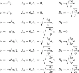
Solution of this algebraic system for ν, A0, A1, A2, B1 and B2 gives

ν = −8a2q+pA0, A1 = 0, A2 = −

12a2_q

p , B1 = 0, B2 = 0 ν = −5a2q+pA0, A1 = 0, A2 = −

6a2_q

p , B1 = 0, B2 =

6a2_q p i

ν = −5a2q+pA0, A1 = 0, A2 = −

6a2_q

p , B1 = 0, B2 = −

6a2_q p i

(20)

where a, A0 arbitrarily chosen constants and i =

√

−1. The real solution of the conformable KdV equation is expressed as

u1(z, t) = A0−

12a2_q p tanh

2

a(z+ (8a2q−pA0) tγ

γ)

(21)

for arbitrary a 6= 0 and A0. On the other hand, the complex solutions are

repre-sented as

u2,3(z, t) = A0−

6a2_q p tanh

2

γ)

± 6a

2_q

p tanh

γ)

sech

γ)

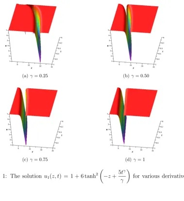
(22) The real valued exact solution is pictured out in Fig 1(a)-1(d) for various derivative orders in a finite domain of z and t. This solution is a particular form of u1(z, t)

determined by assuming A0 = 1, a = −1, q = −1/2, p = 1. These parameters

(8)

(a) γ= 0.25 (b) γ= 0.50

(c) γ= 0.75 (d)γ= 1

Figure 1: The solution u1(z, t) = 1 + 6 tanh2

−z+ 5t

γ

for various derivative orders

5 Solutions to the conformable time fractional

mKdV Equation

The fractional traveling wave transform (6) reduces the mKdV equation (2) into

−aν U0 +apU2U0+qa3U000 = 0 (23)

where 0 denotes the classical derivative with respect to η. s is determined as 1 by balancing U2U0 and U000. Thus, the predicted solution is set as

(9)

Substitution of this solution into (23) reads

a3qB1+apA12B1

sin (w(η)) (cos (w(η)))3 + −4a3qA1−apA13+ 2apA1B12

(sin (w(η)))2(cos (w(η)))2 + 2 (cos (w(η)))2apA0A1B1sin (w(η))

+ −5a3qB1−2apA12B1+apB13

(sin (w(η)))3cos (w(η)) + −2apA0A12 + 2apA0B12

(sin (w(η)))2cos (w(η)) + apA02B1−aν B1

sin (w(η)) cos (w(η)) + 2a3qA1−apA1B12

(sin (w(η)))4 + −apA02A1+aν A1

(sin (w(η)))2

−2 (sin (w(η)))3apA0A1B1 = 0

(25)

Some algebra and equating the coefficients of sin and cos functions to zero leads the following algebraic system:

−aA1 6a2q+pA12−3pB12

+ 8a3qA1−apA02A1+apA13−4apA1B12+aν A1 = 0

−2apA0A1B1 = 0

6a3qB1+ 3apA12B1 −apB13 = 0

4apA0A1B1 = 0

−5a3qB1 +apA02B1−2apA12B1 +apB13−aν B1 = 0

6a3qA1 +apA13 −3apA1B12 = 0

2apA0 A12−B12

= 0

−2apA0 A12−B12

= 0

−14a3qA1+apA02A1−2apA13+ 7apA1B12−aν A1+aA1 6a2q+pA12−3pB12

(10)

Solving this system for a, ν, A0, A1 and B1 gives the solution set

ν =a2q, A0 = 0,A1 = 0, B1 = r

6q p a

ν =a2q, A0 = 0,A1 = 0, B1 =− r

6q pa

ν =−a2q, A0 = 0,A1 = r

−6q

pa, B1 =0 ν =−a2q, A0 = 0,A1 =−

r

−6q

pa, B1 =0 ν =−a2q/2, A0 = 0,A1 =

r

−3q

2pa, B1 =

r

3q

2pa ν =−a2q/2, A0 = 0,A1 =

r

−3q

2pa, B1 =−

r

3q

2pa ν =−a2q/2, A0 = 0,A1 =−

r

−3q

2pa, B1 =

r

3q

2pa ν =−a2q/2, A0 = 0,A1 =−

r

−3q

2pa, B1 =−

r

3q

2pa

(27)

for arbitrary constant a. Thus, the solutions in both real and complex forms are constructed as

u4,5(z, t) =± r

6q

p asecha(z−a 2

qt

γ

γ) u6,7(z, t) =±

r

−6q

p atanha(z+a 2_qtγ

γ) u8,9(z, t) =

r

−3q

2p atanha(z+ a2_q

2

tγ

γ)±

r

3q

2pasecha(z+ a2_q

2

tγ

γ) u10,11(z, t) =−

r

−3q

2p atanha(z+ a2q

2

tγ γ)±

r

3q

2pasecha(z+ a2q

2

tγ γ)

(28)

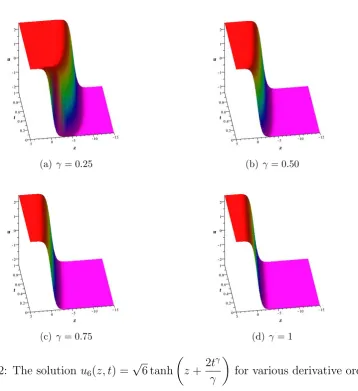
for arbitrary a. A particular form of the solutionu6(z, t) (the positive signed one)

(11)

(a) γ= 0.25 (b) γ= 0.50

(c) γ= 0.75 (d)γ= 1

Figure 2: The solution u6(z, t) =

√

6 tanh

z+2t

γ

for various derivative orders

6 Conclusion

(12)

References

[1] Boussinesq, J. (1877), Essai sur la theorie des eaux courantes, Memoires pre-sentes par divers savants l’Acad. des Sci. Inst. Nat. France, XXIII, pp. 1-680. [2] Korteweg, D. J., de Vries, G. (1895), ”On the Change of Form of Long Waves Advancing in a Rectangular Canal, and on a New Type of Long Stationary Waves”, Philosophical Magazine, 39 (240): 422-443.

[3] Miura, Robert M., Gardner, Clifford S., Kruskal, Martin D. (1968), ”Korteweg-de Vries equation and generalizations. II. Existence of conservation laws and constants of motion”, J. Mathematical Phys., 9 (8): 1204-1209. [4] Wadati, M., & Toda, M. (1972). The exact N-soliton solution of the

Korteweg-de Vries equation. Journal of the Physical Society of Japan, 32(5), 1403-1411. [5] Hirota, R. (1971). Exact solution of the Korteweg-de Vries equation for

mul-tiple collisions of solitons. Physical Review Letters, 27(18), 1192.

[6] Wazzan, L. (2009). A modified tanh-coth method for solving the KdV and the KdV-Burgers’ equations. Communications in Nonlinear Science and Nu-merical Simulation, 14(2), 443-450.

[7] Wang, M., Li, X., & Zhang, J. (2008). The (G’/G)-expansion method and traveling wave solutions of nonlinear evolution equations in mathematical physics. Physics Letters A, 372(4), 417-423.

[8] Zheng-De, D., Zhen-Jiang, L., & Dong-Long, L. (2008). Exact periodic solitary-wave solution for KdV equation. Chinese Physics Letters, 25(5), 1531. [9] L¨u, D., Cui, Y., L¨u, C., & Wei, C. (2010). Novel composite function solu-tions of the modified KdV equation. Applied Mathematics and Computation, 217(1), 283-288.

[10] Wazwaz, A. M. (2004). A sine-cosine method for handling nonlinear wave equations. Mathematical and Computer modeling, 40(5-6), 499-508.

[11] He, J. H., & Wu, X. H. (2006). Exp-function method for nonlinear wave equations. Chaos, Solitons & Fractals, 30(3), 700-708.

(13)

[13] Korkmaz, A., & Hosseini, K. (2017). Exact solutions of a nonlinear con-formable time-fractional parabolic equation with exponential nonlinearity us-ing reliable methods. Optical and Quantum Electronics, 49(8), 278.

[14] Hosseini, K., & Ansari, R. (2017). New exact solutions of nonlinear con-formable time-fractional Boussinesq equations using the modified Kudryashov method. Waves in Random and Complex Media, 1-9.

[15] Korkmaz A., On The Wave Solutions of Conformable Fractional Evolution Equations, Commun. Fac. Sci. Univ. Ank. Series A1, 67(1) 68-79, 2018. [16] Korkmaz A., Exact Solutions to (3 + 1) Conformable Time Fractional

Jimbo-Miwa,Zakharov-Kuznetsov and Modified Zakharov-Kuznetsov Equa-tions, Communications in Theoretical Physics, 2017, 67(5), 479-482.

[17] Kaplan, M., & Hosseini, K. (2018). Investigation of exact solutions for the Tzitz´eica type equations in nonlinear optics. Optik-International Journal for Light and Electron Optics, 154, 393-397.

[18] Hosseini, K., Mayeli, P., & Ansari, R. (2017). Bright and singular soliton solu-tions of the conformable time-fractional Klein-Gordon equasolu-tions with different nonlinearities. Waves in Random and Complex Media, 1-9.

[19] Hosseini, K., Mayeli, P., & Ansari, R. (2017). Modified Kudryashov method for solving the conformable time-fractional Klein-Gordon equations with quadratic and cubic nonlinearities. Optik-International Journal for Light and Electron Optics, 130, 737-742.

[20] Kaplan, M., Mayeli, P., & Hosseini, K. (2017). Exact traveling wave solutions of the Wu-Zhang system describing (1+ 1)-dimensional dispersive long wave. Optical and Quantum Electronics, 49(12), 404.

[21] Tasbozan, O., C¸ enesiz, Y., & Kurt, A. (2016). New solutions for conformable fractional Boussinesq and combined KdV-mKdV equations using Jacobi ellip-tic function expansion method. The European Physical Journal Plus, 131(7), 244.

[22] C¸ enesiz, Y., Tasbozan, O., & Kurt, A. (2017). Functional Variable Method for conformable fractional modified KdV-ZK equation and Maccari system. Tbilisi Mathematical Journal, 10(1), 117-125.

(14)

[24] Abdeljawad, T. (2015). On conformable fractional calculus. Journal of com-putational and Applied Mathematics, 279, 57-66.