Mean control charts for multivariate normal processes

VICTORIA ~ UNIVERSITY

•

' : n

& z 0 ~ 0 0 ~

DEPARTMENT OF COMPUTER AND

MATHEMATICAL SCIENCES

Mean Control Charts for Multivariate

Normal Processes

Pak Pai Tang

(54EQRM 15)

May, 1995

(AMS: 62N10)

TECHNICAL REPORT

VICTORIA UNIVERSITY OF TECHNOLOGY

(P

0

BOX 14428) MELBOURNE MAIL CENTRE

MELBOURNE, VICTORIA, 3000

AUSTRALIA

Mean Control Charts for Multivariate

Normal Processes

PAKFAITANG

Victoria University of Technology, Melbourne, Australia.

ABSTRACT

Some methods for monitoring and controlling the mean level of a multivariate normal process are presented in this paper. Those that do not depend on prior estimates of the process parameters are particularly attractive to short-run or low volume manufacturing environments. As the given techniques involve sequences of independent or approximately independent standard normal variables, the resulting control charts can all be plotted using the same scale irrespective of product types, thus simplifying charting administration. A simulation study indicates that these control procedures are particularly useful for 'picking up' a sustained shift in the process mean vector when subgroup data are used, even if prior information about the process parameters are not available. Some illustrative examples are presented.

INTRODUCTION

In many industrial situations, it is not uncommon to monitor on-going performance of a production process with respect to more than one process or product characteristic simultaneously. If the product characteristics are correlated and no consideration is made of their joint distribution, the use of separate control charts for each of them can be misleading. Specifically, the related variables, when studied separately, may appear to be in statistical control while in fact the manufacturing system is out-of-control or vice versa when considering the quality characteristics in their multivariate context. Montgomery et al.(1972) and Alt et al.(1990) illustrated this for the case of p = 2 variables. Under these circumstances, it seems reasonable to consider the use of multivariate quality control procedures which take into account the covariance structure of the quality characteristics.

Most of the statistical process control (SPC) techniques proposed to date for controlling the mean of a multivariate normal process are based on Hotelling's (1947)

z

2 or

Doganaksoy et al.(1991), Hawkins (1993) and Hayter et al. (1994)). However, all of this work essentially assumes that the process mean (or target) µ and the process covariance matrix ~ are known or that they can be reliably estimated based on sufficient data prior to full scale production. Thus, these techniques do not readily lend themselves to applications in the short-rui:i or low-volume manufacturing environment where data for estimating the process parameters are usually scarce or unavailable.

The main purpose of this paper is to present some 'self-starting' and unified procedures for controlling the mean vector of a multivariate normal process where prior estimates of the process parameters are not available such as frequently occurs in short-run, low-volume and multi-product manufacturing environments. The proposed techniques also facilitate the control of long-run processes at an earlier stage when the process parameters have to be estimated from the data stream of the current production. For completeness, control procedures are also given for the cases where µ,

L

or both are assumed known in advance of the production runs.

In addition to this introduction, the paper is organized into five sections. In the next section, control statistics for use with individual and subgroup data are given according to various assumptions about the knowledge of the process parameters. Some numerical examples illustrating the use of these techniques are provided in section 3. In s,ection 4, simulation results are presented and statistical performance of the proposed techniques discussed. A brief account of the computational requirements for implementation of the proposed techniques is given in section 5. The final section concludes with a brief summary and further remarks. The total discourse is in the context of discrete items manufacture.

MULTIVARIATE MEAN CONTROL CHARTS

Like the 'Q' charting approach previously proposed by Quesenberry (1991) for controlling univariate normal processes, the techniques presented in this paper involve the use of the probability integral tramformation of some (scaled) quadratic forms in order to produce sequences of independent or approximately independent standard normal variables. These procedures essentially enable charting to commence with the first units or samples of production whether or not prior knowledge of the process parameters is available. For the case where no relevant data is available prior to a production run, the process parameters µ and ~

are 'estimated' and 'updated' sequentially from the current data stream. These dynamic estimates, together with the next observation or subgroup are in turn used to determine whether the process remains stable.

The appropriate control statistics based on both individual observations and subgroup data are presented in the following subsections. The control statistics are given for the cases when both, either or neither of the process parameters µ and

L

are assumed known in advance of the production run.

(a) Control Charts Based on Individual Measurements

Further, let Xk, Sk and Sµ.k denote respectively the mean vector, the usual and the

'mean-dependent' covariance matrix of the first k observations as defined below :

These values can be updated sequentially using the following recursive formulae :

The following additional notation will be used.

<I>{•) :

distribution function of a standard normal variable

<1>-1 ( • ) : inverse of the standard normal distribution function

k = 2,3, ... .

k = 3,4, ... .

k = 2,3, ... .

x~(.)

:

distribution function of a chi-square variable with v degrees of freedom

Fvi

,

v

2 ( • ) : distribution function of an

F

variable with v 1 numerator degrees of freedom

and v2 denominator degrees of freedom

The appropriate control statistics are now presented as follows:

Case

CD :

Both µ and

L

known

zk

=

<1>-

1

[x~C4)]

k

=

1,2, ... .

where

4

=

(xk -

µ)'

L-'(xk -

µ)

(1)

Case OD : µ unknown,

L

known

zk

= <1>-1

[x!C7k>]

k

=

2,3, ... .

Case

(flD :

µ known,

L

unknown

For this case, two alternative control statistics are considered which, as demonstrated later, have slightly different performance. They involve the use of Sµ,k and Sk respectively.

(a) Uses µ in

L

estimate

k=p+l, ... .

(3a)

(b) Uses Sample Variance-Covariance Matrix

k = p+2, ... .

Where T. -k -

(k-1-p)(x

p(k-2) k - µ

)'s-1 (x

k-1

k - µ

)

(3b)

Case CM : Both µ and

L

unknown

k = p+2,. ...

Where T. _ k -

(ck-I

kp(k-2)

X

k-1-p))(x

k -

x )'s-1 (x x )

k-1

k-1

k -

k-1

(4)

Note that for the cases with some unknown parameters, monitoring the process can essentially commence with the first units of production without having to wait until enough process performance data has built up. This is crucial for the control of short-run processes and processes during 'wann up'.

As shown above, for case (I), a value of Zk corresponds to Xk for all values of

k = 1,2,. ... However, no value of Zk corresponding to the first observation X₁ is calculated for case (II). This is due to the fact that the unknown process mean vector µ has to be estimated from X₁ before its constancy can be subsequently monitored, based on further observations. For case (III), if the control statistics given by (3a) are used, the monitoring procedure begins after p +I observations. For the remaining cases, control is initiated at the (p

+

2)th observation.

In

general, if

L

has to be estimated from the current data stream, the starting periods of the control procedure are such that they yield positive definite estimates of

L.

For example, no value is plotted using the control statistics of (3b) or (4) prior to the (p

+

2)th observation because the sample covariance matrix Sk-I , used in the formula, is not

of full rank and hence is not invertible fork less than p

+

2.

Except for (3b),

{zk}

for each case is a sequence of independently and identically

distributed (i.i.d) normal variables with mean 0 and standard deviation I under the stable

first 50 p-variate measurements was simulated for p = 2, 3 and 5 based on 10,000 runs when either 3-sigma limits or only the upper 99.73th probability limit is used. The results appear to agree well with the nominal value of 1-0.997350 = 0.1264. The reason the above criterion is chosen as a measure of in-control performance instead of the usual average run length is that the control statistics given by (3b) are primarily concerned with short production run situations in which the total number of observations rarely exceeds 50.

As the plot statistics for all cases are sequences of independent (or approximately independent) standard normal variables, the resulting control charts can be constructed using the same scale and with the same Shewhart control limits ±3. In addition, supplementary run rules can be employed to reveal any assignable causes hidden in the point patterns of the charts. Although the argument statistics ~ 's can be plotted instead of the transformed variables Zk' s, this practice is not recommended if additional computational effort can be justified. This is because, for those cases other than case (I), the use of

lie'

s results in varying control limits which can lead to misinterpretation. The use of these procedures is illustrated after the appropriate control statistics based on subgroup data have been presented.

(b) Control Charts Based on Subgroup Data

In practice, the use of subgroup data is often preferable to individual measurements even in situations where only a limited amount of data are available. This is justified on the basis that the resulting control charts are more sensitive to substantial shifts in the process average and that the subgroup mean (vector) is less affected by departure from the underlying normality assumption, by virtue of the central limit theorem.

A little adaptation of the above formulae yields appropriate control statistics for monitoring the stability of the process mean vector based on subgroup data. Discussion will be restricted to the case of constant subgroup size, as this is a common phenomenon. Let Xij, n

where s~> = S~~

1

•

4

=

0. The same technique is now applied to transform the sample mean

vectors X(;) 's to standard normal variables for each of the cases considered above for the individual measurements.

Case

CD :

Both µ and

L

known

Zk

=

<t>-'[x.!(Tk)]

k = 1,2, ... .

where

4

= n(Xck) -

µ)'

L-

1

(x(k) -

µ)

(5)

Case (Il) : µ unknown,

L

known

k = 2,3, ... .

where

4

= (

nc~-l)

)( x(k) -

Xck-J)}

L-

1

(xck> - Xck-I))

(6)

Case

Cnn :

µ known,

L

unknown

Two alternative techniques which employ different process covariance matrix estimates will be considered for this case. The first one incorporates µ into its 'running' estimate of

L

whereas the other one is based on the pooled estimate S~l

1

•

4

. It will be seen in section 4 that these control procedures have comparable performance.

(a) Uses µ in estimation of

L

k = 2,3,... , n ~

p

(7a)

(b) Uses Pooled Sample Covariance Matrix

Zk = <t>-1[Fp,k(n-I)-p+t

(T,J]

k = 1,2,... , n > p

Where

4

= [

n[k~~(::.=;~+l]](

x(k) - µ )' (

s~

)-I (

x(k) -

µ)

(7b)

Case

CM :

Both µ and

L

unknown

k = 2,3, ... . ,n> p

where

T.

-(nCk-IXkCn-l}-p+i>)(x - X

)'(s<k> )-

1( x - X ) (8)

Under the assumption that the Xu 1

s are independent observation vectors obtained from

a common process with a NP(µ,

L)

distribution, the control statistics given by ( 5), ( 6) and

(7a) are sequences of independently distributed standard normal variables (see Appendix A). For those given by (7b) and (8), successive plotted values also arise from a standard normal distribution but they are correlated due to the use of the pooled sample covariance matrix. Sequences of independently distributed variables can be obtained for these latter cases by replacing the pooled sample covariance matrix S~':liet1 by the sample covariance matrix of the

current subgroup, S(k). This is not considered, however, because it is found that the

performance of the resulting charts are poor even when some additional run rules are used. Furthermore, ignoring the issue of correlation does not appear to have remarkable effect on the false signal rates for the control techniques based on statistics (7b) and (8).

A remark should be made about the computation of the argument statistics for (1) - (8) above which involve evaluation of the inverse of a matrix. In fact, each of these arguments can be expressed as a quotient of two determinants, thus eliminating the need for inverting either the known process covariance matix or some estimates of it (see for eg., Morrison (1976), p.134 ). For instance, the argument statistic of (4) has the following alternative expression

I

s

(k-l)(k-1-p)

(x x )(x x

)'I

k-1

+

kp(k-2) k - k-1 k - k-1

~

=

I I

- i

sk-1

Evaluating an expression of this form is much more convenient than that of its original form especially when the number of quality characteristics, p is large.

For some general guidelines on using the above control charting approach and a discussion of its advantages and disadvantages, readers are referred to the article by Quesenberry (1991) from which the ideas of this present work originate.

EXAMPLES

In this section, use of the proposed techniques are illustrated by some numerical examples based on simulated data as well as using data from a previously published article. The examples presented here are not intended to cover all possible situations, however, they provide some insight into the behaviour of the proposed techniques under various circumstances.

Example 1

The first illustration uses the formulae for individual measurements. 30 observations have been generated from a bivariate normal distribution with the following parameters

( I 1.275]

L

= 1.275 2.25 .

IE. It should be noted that the use of 3- () control limits in this and subsequent examples is merely for the purpose of illustration. In practice, it may be preferable to use narrower control limits or only the upper control limit in line with the traditional Hotelling T2 charting approach.

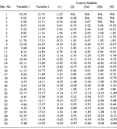
TABLE 1. Simulated Data and Values of The Control Statistics based on Individual

Measurements for Example 1

Control Statistic

Obs. No. Variable 1 Variable 2 (1) (2) (3a) (3b) (4)

1 10.39 15.70 -1.27 NA NA NA NA

2 9.02 14.19 -0.08 -0.28 NA NA NA

3 9.28 13.71 -0.50 -0.62 0.07 NA NA

4 . 8.67 14.04 0.61 -0.19 0.52 0.06 -0.32

5 9.22 14.99 0.40 -0.55 0.46 0.24 -0.21

6 8.82 11.54 1.98 1.99 2.09 1.64 1.56

7 9.07 14.14 -0.24 -1.39 -0.37 0.17 -1.52

8 11.70 17.31 0.73 1.50 0.47 1.29 1.83

9 10.92 16.35 -0.35 0.22 -0.60 -0.57 -0.07

10 9.64 14.84 -1.15 -1.80 -1.21 -1.24 -1.91

11 8.31 12.85 0.70 0.18 0.45 0.44 -0.01

12 9.56 14.23 -1.16 -1.55 -1.29 -1.30 -1.56

13 10.39 14.74 -0.22 0.15 -0.14 -0.16 0.19

14 10.11 15.84 -0.43 -0.30 -0.36 -0.42 -0.33

15 9.53 13.79 -0.42 -0.57 -0.39 -0.44 -0.55

16 11.15 16.77 0.05 0.46 0.01 0.06 0.45

17 8.03 11.89 1.24 0.88 1.05 1.03 0.72

18 9.68 14.04 -0.67 -0.86 -0.62 -0.66 -0.72

19 9.57 14.11 -0.95 -1.48 -1.00 -1.00 -1.39

20 9.05 13.58 -0.29 -0.98 -0.40 -0.38 -1.01

21 12.40 18.15 1.59 1.98 1.37 1.49 1.80

22 10.17 15.17 -2.14 -1.37 -2.12 -2.13 -1.49

23 8.41 13.00 0.58 0.22 0.38 0.37 0.07

24 10.31 16.11 -0.33 -0.07 -0.03 -0.06 0.08

25 9.66 13.57 0.19 0.05 0.55 0.50 0.44

26 9.50 13.78 -0.44 -0.80 -0.35 -0.36 -0.62

27 10.91 17.65 1.22 1.44 1.40 1.38 1.52

28 10.59 16.43 -0.20 0.03 -0.23 -0.25 -0.11

29 9.71 14.05 -0.62 -0.73 -0.54 -0.56 -0.55

"'

...

i ....

..

_.lll

GD ₀

g c 0 0 ~ 'f 'I' "'

..

"' 0 ~ 'I 'I' +

0 IO 15 20 25 30

Observation numller

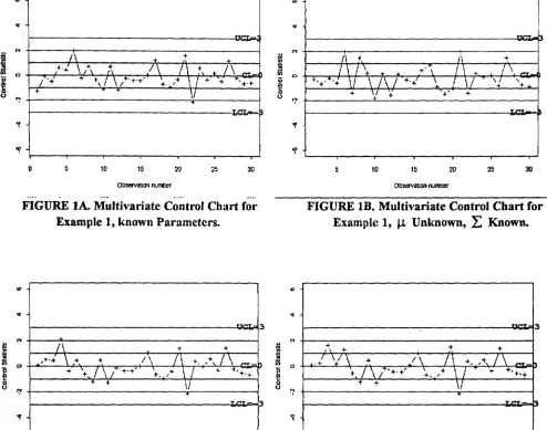
FIGURE lA. Multivariate Control Chart for

Example 1, known Parameters.

,+·+ I

5 10 15 20 25 30

Observation number

3

FIGURE 1C. Multivariate Control Chart for

Example 1, µ Known,

:L

Unknown, Statistic (3a).

"'

"'

u "'

i

~ _c 0

"

."'!

'I

"

5 10 15

"' ... "' c "! 'I ~

10 15 20 30

Observation number

FIGURE lB. Multivariate Control Chart for

Example 1, µ Unknown,

:L

Known.

I ·+·+'

10 15 20 25 30

ObServation number

FIGURE lD. Multivariate Control Chart for

Example 1, µ Known,

L

Unknown, Statistic (3b).

+

+' ₊

20 25 30

Observation number

Note that for the cases with some unknown parameters, the corresponding statistics were computed using the values of µ and

.L

as given above. Note also that since p = 2, calculations of the plotted values of the control statistics (2), (3a), (3b) and ( 4) have been started with the 2nd, 3rd, 4th and 4th observations respectively. The latter statistic is particularly·useful as it enables exercise of control over new, start-up or short-run processes without requiring accumulation of a considerable amount of process data for estimation of the unknown parameters.

As shown in the figures, none of the plotted points exceed the control limits for each of the control charts. This is as expected because the data for this example can be regarded as having been collected from an in-control process. It is also interesting to note that after the first few observations, the movement of the charted points are very similar for all cases. This is especially true for the two charts based on formulae (3a) and (3b ). This phenomenon is typical for in-control multivariate normal processes.

Example 2

Next, to demonstrate the behaviour of the control charts based on subgroup data for a stable process, 120 observations have been generated from a trivariate normal distribution with

and

(

0.0625 0.1062. 5 0.0. 5

J

.L

= 0.10625 0.25 0.136

0~5 0.136 0.16

These observations are grouped into samples of size n = 4 and the corresponding values of the control statistics (5), (6), (7a}, (7b) and (8) were calculated and plotted in Figures 2A to 2E.

Note that except for the case with known parameters and when the statistic (7b) is used, charting begins with the 2nd subgroup.

"

ll

""

..

!il 0 ~ 0 0 .,

..

... 0 I '

'"! +'

'i

'\'

0 5 10 15 20 25 30

Subgroup Number

FIGURE 2A. Multivariate Control Chart for Example 2, Known Parameters.

Subgroup Number

3

FIGURE 2C. Multivariate Control Chart for

Example 2, µ Known,

L

Unknown, Statistic (7a) .

.,

..

"'

v

~

Iii 0

i5 _\

€ _c

tJ '"!

"f

"!

5 10 15

IP

..

... 0 T· '"! 'i '\'

10 15 20 25 30

Subgroup Number

FIGURE 2B. Multivariate Control Chart for

Example 2, µ Unknown,

L

Known.

..

"'

+

0

+,I\ I .+

'"!

..,

"1

10 15 20 25 30

Stllgroup NUmber

FIGURE 2D. Multivariate Control Chart for

Example 2, µ known,

L

Unknown, Statistic (7b).

2D 25 30

Subgroup Number

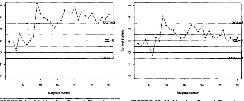
Example 3

In this example, two charts are shown in order to compare the control techniques based

on subgroup data for the cases when the parameters µ and

L:

are assumed known and when

they are both unknown. Figures 3A and 3B show these control charts for 30 samples of 3

observations each from a bivariate process where the mean of the 1st variable increases by 1.5

standard deviations after the 8th sample. The first 8 samples were generated from a N₂

(µ

,

L:)

process distribution with

µ=G~J

and = ( 0.25 0.375)

L:

0.375 I

whereas samples 9 to 30 were simulated from N ₂ (µnew,

L:}

where

= (10.75)

µnew 23 .

Note that the correct values of µ and

L:

to use for computing statistic (5) are those

before the shift occurs. The figures show that whilst the shift is large enough to trigger

out-of-control signals from both charts as soon as subgroup 9 is observed, that based on unknown parameters gradually settles into a pattern indicative of in-control conditions. This is due to the fact that the corresponding control statistic utilizes the current data stream to estimate the unknown values of the process parameters sequentially, causing the effect of parameter changes to 'dilute' as more out-of-control data are incorporated into the parameter estimates. It should be noted, that if an outlier or out-of-control observation (or subgroup) is present,

that observation should be removed from subsequent computations. If this is not done, the

parameter estimates will be distorted, causing an out-of-control process to appear in-control or

vice versa.

u 1i: "' ~ e ~ 0 0 IO ...

/\

+ + + I' +

+

I

_·+

\r

_{+ +}

' _+. +./\ +. /

+.+ + + +. I .!"_. -.

\ I

N ...

... I

0

(\ +

... _' r T

-\ I ' ₊ ,

"

":' +

-'f

'I'

0 10 15 20 30 Subgroup Number

FIGURE JA. Multivariate Control Chaa1 for Exarn1>le 3, Known Parameters.

IO

..

~ N

~ 0 ~ 0

0

":'

'I

'!'

+

J\

--I +

' +.+ +

I •T\

+ + \ ,+, /_T\

+_! T,+·+' ₊ + .. + .. T \

.,+,_j-+ . ...' \ I T

\/

+

--5 10 15 20 25 30

Subgroup Number

FIGURE 3B. Multivariate Control Chart for Example 3, Unknown Parameters.

Example 4

As a preliminary investigation of the effect of changes in process standard deviations on the individual values control charts, 3 0 observations are considered that have been generated fron:i a trivariate normal process where the standard deviations of two of the variables double after the 13th observation. Observations 1 to 13 were generated from N₃

(µ,L)

with

and

( 0.01

L=

0.042

0.0825

0.042 0.0825] 1.44 -0.18

-0.18 2.25

while the remaining subsequent observations were generated from N₃

(µ,

Lnew)

where

(

0.01 0.084 0.165]

Lnew

= 0.084 5.76 -0.72

0.165 -0.72 9

The individual values control charts for the case when both or neither of the process

parameters are assumed known were constructed based on these simulated data and these are displayed in Figure 4A and 4B respectively. As shown in the figures, the change in the process standard deviations causes a spike on both the control charts at the 21st observation. However, the signal from the latter is less pronounced than that corresponding to the known parameter case. This example demonstrates that the individual values control chart which does not assume known values of the process parameters can also be used to detect changes in the process covariance matrix

L.

"

t;

'"'

m

~ 0 u

"'

.,

\

+ + • • - T ...

"' _J\ + \ ' ₊ , /\ _I

C> ~ +, + /" ~ I \ .+ + \ /l

-\ I + \ •. +·+·..! \} ~ + +

T ₊

~

T~T-.,

~

5 10 15 20 30

Observation number

FIGURE 4A. Multivariate Control Chart for Example 4, Known Parameters.

10 15 20 30

ObseMilicn number

Example 5

To see how the control technique with unknown parameters that is based on subgroup data performs in comparison to an existing method, consider the data given by Alt et al.(1976). These authors presented formulae to compute the control limits for the

T

2 -type control chart based on a small number of subgroups, both for retrospective and future testing of the mean level of a multivariate normal process and used the data to illustrate the use of these so-called

small sample probability limits. The data consists of measurements on p = 2 quality characteristics which are grouped into subgroups of size n = 10. Due to limited space, the summary data are not reproduced here. However, for ease of comparison, the values of the T2-type statistic, the stage 1 (retrospective) and stage 2 (future) control limits are given in TABLE 2, together with the results obtained using the technique (8) proposed in this paper. Note that the stage 1 and stage 2 control limits are set at ex.= 0. 001 and ex.= 0. 005 respectively.

TABLE 2. Values of Alt et al.'s Test Statistic, Small Sample Probability Limits and Control Statistic (8) for Example 5.

Subgroup Alt et al. 's Stage 1 UCL

Revised Value of Alt et al. 's Control Statistic

Revised Stage 1 Control Statistic

No. Stage 1

Control Statistic

1 0.009 1.3268

2 1.147 1.3268

3 0.136 1.3268

4 4.901* 1.3268

5 0.632 1.3268

Subgroup Alt et al.'s Stage 2

No. Stage 2

i

UCLt

Control Statistic

6 0.392 1.5906

7 0.197 1.5906

8 4.594* 1.5906

9 0.190 1.5906

10 0.226 1.5906

11 0.410 1.5906

12 0.460 1.5906

0.327 0.264 0.034 NA 0.057

UCL (8)

0.9546 0.9546 0.9546

0.9546

NA 1.0758 -1.4909 5.0192* -0.5821t

0.7766 0.5906 4.8528* 0.404St 0.3248

1.0596 0.9490

* These numbers exceed their respective UCLs indicating the presence of assignable causes.

t

These and subsequent values are calculated after removing the out-of control subgroups immediately preceding them.

: These are based on subgroups 1, 2, 3 and 5.

CONTROL PERFORMANCE

It is shown in Appendix B, that the statistical performance of the techniques presented above depend on the following parameter(s) (scalar, vector or matrix) for each of the given types of process changes (besides the change point r) :

(a) A sustained shift in the Mean Vector from µto µnew whilst L remains unchanged,

(b) A sustained shift in Covariance Matrix from L to Lnew whilst µ remains unchanged,

(c) A simultaneous sustained shift in Mean Vector from µto µnew and Covariance Matrix from L to Lnew ,

and

I

Note that

:L

2 _{here denotes the symmetric square root matrix of}

_L

_{such that}

:L=:L~:L~

(see Johnson et al.(1988), p.51) and

:L-~ =(:L~r

1

•

The importance of these results is clear when one realizes that the effort for determining the control performance of the proposed techniques is greatly reduced. For instance, in order to determine the performance under the first type of process changes, it may be assumed, without loss of generality, that

µ

=

(0,0, ... ,0)', L =I and µnew subsequently considered in the form of µnew= (A.,0, ... ,0) for various values of A. .

In this section, we will consider only the simplest type of process changes, namely, a persistent change in the process mean vector. The performance of the proposed techniques are evaluated on the basis of probability of detection within m = 5 successive observations or subgroups by means of simulation. This is chosen as the performance criterion instead of the common measure of ARL because, as demonstrated in the examples using simulated data, the first few observations or subgroups after the change appear to predominantly determine whether those techniques with unknown parameters are capable of 'picking up' the shift. In

other words, if the mean shift is not detected within the first few observations or subgroups after its occurence, it is even more unlikely that this will be 'picked up' by subsequent observations or subgroups because of the 'diluting' effect. Another reason is, the run length distributions for the techniques with some unknown parameter are not geometric so that ARL is clearly not a suitable performance criterion (see Quesenberry ( 1993) ). Furthermore, this paper is particularly concerned with short production runs or low volume manufacturing and as such early response of the techniques to any process anomalies or irregularities is a crucial factor.

It should be pointed out that only an upper control limit is used in the simulation. This is chosen because the control techniques are intended primarily for 1

large values for the control statistics. However, in practice, it might be preferable to use both the lower and upper control limits because the former can provide protection against occasional changes in the variance-covariance matrix and other process disturbances which may cause abnormally small values for the control statistics. The limit is set at the 99.73th percentage point so that the false alarm rate for the proposed techniques equates to that of the traditional Shewhart charts with 3-sigma limits. As a partial check of the simulation, we have included results for those cases with known parameters.

The results for the individual values control techniques obtained through 10,000 simulation runs are tabulated in TABLE 3 for various combinations of p, A. and r. In TABLE 4, the results for those techniques based on subgroup data are given. Note that the subgroup size used in each case is n = p

+

1 . This is the minimum common sample size that must be used if

L

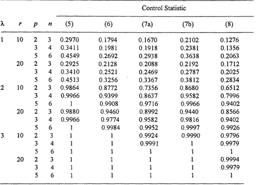
is unknown except for technique (7a). Note also that, the exact probabilities for techniques (1) and (5) are obtainable from the noncentral chi-square distribution tables or standard statistical software packages. The simulation results for these techniques are found to agree well with the theoretical values. For instance, the theoretical probabilities for technique (I) are 0.0569, 0.3452, 0.8571 and 0.9972 respectively for A.= 1, 2, 3 and 4 when p = 3. These are very close to the corresponding figures in Table 3.

As shown in TABLE 4, the control techniques based on subgroup data for the cases with at least some unknown parameters can be expected to perform as well as the technique with known parameters under this type of process change especially when the noncentrality parameter, A. is larger than or equal to 2. For instance, using control statistic (7b) and (8) with a subgroup size of n

=

6 when p

=

5, the probabilities of 'picking upr a mean shift of A.

=

2 which occurs after the 10th subgroup, within 5 consecutive subgroups, are respectively 0.9966 and 0.9402. For smaller values of A., these control techniques can also be expected to perform reasonably well relative to the technique corresponding to the known parameter case. For example, these probabilities are 0.3812 and 0.2834 respectively when statistics (7b) and (8) are used, as compared to 0.4513 for the known parameter case. As for control based on individual observations, those techniques with some unknown parameters have poor performance relative to that based on known parameters when A. and r are small and p is large. However, the performance of these individual values control charts improve with increasing value of A. and

r.

As shown in Table 3, the probability of detecting a shift of A.= 5 for a bivariate process within 5 successive observations using statistic ( 4) which does not assume known values for

TABLE 3. Probability of Detection Within m = 5 Subsequent Observations.

Control Statistic

A. r p (I) (2) _(3a)" (3b) (4)

1 10 2 0.0720 0.0492 0.0328 0.0327 0.0245 3 0.0537 0.0399 0.0260 0.0260 0.0223 5 0.0417 0.0306 0.0197 0.0179 0.0172 20 2 0.0736 0.0588 0.0437 0.0432 0.0367 3 0.0545 0.0432 0.0363 0.0364 0.0304 5 0.0403 0.0345 0.0267 0.0265 0.0247 2 10 2 0.4430 0.2560 0.0807 0.0792 0.0541

3 0.3437 0.2033 0.0553 0.0519 0.0364 5 0.2500 0.1428 0.0342 0.0312 0.0228 20 2 0.4357 0.3230 0.1660 0.1702 0.1353 3 0.3456 0.2525 0.1172 0.1164 0.0925 5 0.2508 0.1830 0.0755 0.0746 0.0614 3 10 2 0.9153 0.7050 0.1887 0.1720 0.1325 3 0.8550 0.6014 0.1191 0.1080 0.0827 5 0.7477 0.4752 0.0570 0.0514 0.0408 20 2 0.9124 0.8074 0.4011 0.3976 0.3314 3 0.8533 0.7220 0.2863 0.2854 0.2333 5 0.7530 0.5920 0.1747 0.1662 0.1385 4 10 2 0.9993 0.9687 0.3735 0.3339 0.2728 3 0.9966 0.9354 0.2483 0.2045 0.1967 5 0.9880 0.8762 0.1026 0.0882 0.0722 20 2 0.9994 0.9921 0.7040 0.6954 0.6213 3 0.9960 0.9796 0.5624 0.5548 0.4837 5 0.9900 0.9456 0.3576 0.3482 0.2962 5 10 2 1 0.9996 0.6114 0.5532 0.4880 3 1 0.9982 0.4292 0.3628 0.3076 5 1 0.9930 0.1560 0.1208 0.0984 20 2 1 1 0.9096 0.9004 0.8514 3 1 1 0.8122 0.7986 0.7366 5 0.9999 0.9988 0.5866 0.5630 0.5074

6 10 2 1 1 0.8180 0.7594 0.6980

TABLE 4. Probability of Detection Within m = 5 Subsequent Subgroups.

Control Statistic

A. r p n (5) (6) (7a) (7b) (8)

l 10 2 3 0.2970 0.1794 0.1670 0.2102 0.1276 3 4 0.3411 0.1981 0.1918 0.2381 0.1356 5 6 0.4549 0.2692 0.2938 0.3638 0.2063 20 2 3 0.2925 0.2128 0.2088 0.2192 0.1712 3 4 0.3410 0.2521 0.2469 0.2787 0.2025 5 6 0.4513 0.3256 0.3367 0.3812 0.2834 2 10 2 3 0.9864 0.8772 0.7356 0.8680 0.6512 3 4 0.9966 0.9399 0.8637 0.9582 0.7996

5 6 1 0.9908 0.9716 0.9966 0.9402

20 2 3 0.9880 0.9460 0.8992 0.9440 0.8566 3 4 0.9966 0.9774 0.9582 0.9816 0.9402

5 6 0.9984 0.9952 0.9997 0.9926

3 10 2 3 1 1 0.9924 0.9990 0.9796

3 4 I 1 0.9991 1 0.9979

5 6 1 1 1 1 1

20 2 3 1 1 1 I- 0.9994

3 4 I 1 1 1 0.9979

5 6 I I 1 1 1

COMPUTATIONAL REQUIREMENTS

In this work, evaluation of the standard normal distribution, its inverse, chi-square and

F distribution function are required in order to compute the trasformed

Zk

statistics. In addition, computation of the argument statistics ~ 's involve matrix multiplication and inversion. To implement the proposed control scheme, therefore, requires computing facilities and complex algorithms. Fortunately, these algorithms are widely available and have been built into most of the commercial statistical software packages. The simulated data and the charts in this paper were generated and made by the authour using programs written in S-plus.

CONCLUSIONS AND FURTHER REMARKS

Some methods have been presented for controlling the mean vector of a multivariate normal process. The techniques involve a non-linear probability integral transformation of

costs of charting. Those techniques presented for the case with no prior knowledge of process parameters are particularly attractive for short production runs and low volume manufacturing environments. These control procedures also enable the monitoring of new or start-up processes soon after production commences.

As demonstrated by the examples, the proposed techniques yield similar control chart patterns for a stable in-control process whether or not prior estimates of the process parameters are available. However, for a sustained shift in a parameter, whilst being capable of detecting the change, the control charts based on unknown parameters will eventually settle into an in-control pattern. The sooner the change occurs after the commencement of production, the lower the intensity of the signal and hence it is more likely to go undetected. The last example demonstrates that the control technique based on subgroup data and unknown parameters possesses comparable performance to an existing technique.

The power of the proposed techniques were determined by means of simulation for given sizes of sustained shift in the process mean vector. The results show that the techniques . based on subgroup data have desirable performance whether or not the process parameters are assumed known. in advance of the production run. As for individual values control techniques, the performance of those which do not assume known values for the process covariance matrix

L

or both the process parameters, improves with increasing value of the non-centrality parameter and point at which the change occurs. This is true irrespective of the number of quality characteristics considered.

This paper has been devoted solely to statistical process control and monitoring of the mean of multivariate processes. In practice, it is also of value to monitor the process spread as measured by the variance-covariance matrix

L

which may be subject to occasional changes. Although some methods have been proposed for this purpose (see for eg., Alt et al.(1990)), the assumption is made that

L

is known or can be estimated based on sufficient relevant data. As such, these methods cannot be readily used in manufacturing situations where the total output of the production processes are low. In view of this, efforts should be made to develop new control procedures that do not depend on prior knowledge of

L.

Another issue of practical importance is the identification of variables which are responsible for out-of-control conditions as signalled by the appropriate multivariate control charts. Although this problem has received considerable attention recently, the techniques proposed for this are again based on the assumption that knowledge of

L

is available prior to production.

ACKNOWLEDGMENT

APPENDIX A

Distributional Properties of The Control Statistics

As the arguments involved in establishing the distributio~al properties of all the control statistics are similar, this section will only consider the proof for that given by ( 4). Suppose

X₁,X_{2 , •••} ,X, are independent p-variate random observation vectors which have the same covariance structure and are distributed as

j = 1,2, ... ,r

where ~ denotes the unknown non-singular variance-covariance matrix. Next, define

V =X_{) )} .-X j

=

1,2, . .. ,r

where

- 1 '

X=-LXi.

r j=I

We wish to test the hypothesis

H₀ : µ₁ = µ₂ = ... =µ(say) vs. HA: not all µ/s are equal

Under H₀ and the assumption of a constant process variance-covariance matrix,

where

® denotes the (left) Kronecker Product (see Graybill (1983), p.216) and

.!'.::!. _J_ _l.

r r r

_ l. L::!. _ l.

r r r

C=

_.l .!::l.

r r rxr

Some linear combinations of the p x 1 component vectors VP V2 , •••••• , V, that are

Y1 =a11V1 +a12V2+ ... +a,rVr

y2 = a21 vi + a22 v2 + ... . +a2r vr

In matrix notation, these are represented by the following equation :

Y=rV=(I®A)V

where I is a p x p identity matrix and

A=

Thus,

... a"

Ly=

r:Lvr'

=:L®ACA'

rxr

(Al)

(A2)

Recall that the aim here is to produce vectors Y_1, Y_{2 , •••••• ,} Yr which are uncorrelated. This is the case if A in (A2) is chosen to diagonalize the symmetric matrix C. One choice for A is

A=

I

.Jr

I

J2

I

J6

_ I _ .,/4(4-1)

_ I _ Jr(r-1)

I

.Jr

-I

J2

1

J6

I .,/4(4-1)

0

..1 ₀

J6

I -3

.,/4(4-1) J4(4-I) 0

I

.Jr

0

0

0

-(r-1)

Jr(r-1)

where the rows of the matrix are the normalized eigenvectors of C. Substituting A into (Al)

YI= 0,

Y

2 =

fi-(V

1 -

V

2 ) =

"fi-(X

1 -

X

2 )

Y3

=

-J6{V1

+

v2 -

2V3)

=

-J6(X1

+

x2 -

2X3)

Note that the transformation results in a new set of uncorrelated random vectors Y_{2 ,} Y_{3 , • •••••} ,Yr, one less than the set of original random vectors. This is due to the fact that the transformation is subject to a constraint, namely, the sum of the component vectors V_1, V_{2 , ••••• .,} Vr is equal to a zero vector leading to rank('Lv) = rp - p = r(p-

1).

It is also clear from (A2}that

Lv

is a 'quasi-diagonal' matrix with diagonal submatrices

L

except for the first one which is a zero matrix.

Since the resulting transformed vectors Y_{2 ,} Y_{3 , •••••• ,} Yr are linear combinations of

multivariate normal vectors and

L

v is a quasi-diagonal matrix as mentioned above, they are

mutually independent with common variance-covariance matrix

L .

As the kth observation vector X k, the (k-1 )th sample mean vector X k-i and the sample variance-covariance matrix

based on the first k observations

sk-1

are independent,

I

=

•c~-1)[~

x;

-(k- I)X,

J

(s

k-

ir1[

~x;

-(k-J)X,

J

= (

kkl )(

x

k -

x

k-1)

I (

s

k - 1 )- l (

x

k -

x k-1)

k

=

p

+

2, ... .

are easily seen to be distributed as (Anderson (1984), p.163)

A - (k-2)p F k

(k _

I _

p)

p;k-1- P

To establish mutual independence of successive Ak 's, it is first proved that they are

pairwise independent. Clearly,

are mutually independent. The notation W v

(•IL.)

here denotes the Wishart distribution with v

Thus,

and their independence is preserved. Due to the invariance property of the transformation,

Noting that

(k-2)S* _k-1 = (k-l)S* -_k

y•y•·

_{k k}

and using identity (2.5.6) for matrix inverses (see Press(l 982), Binomial Inverse Theorem,

p.23), Ak may be expressed as follows :

A =

(k-2)

k

(k-1)

_

(v;·(s;)-

1

v;)

2

v;· (s;)

1

v;

+

--'---'----(k -

1)-

v;·(s;)-

1

v;

As

y;'(s:r

1Y; is independent of

s:

(see Srivastava and Khatri (1979), Theorem 3.3.6,

p.94) and

v;+1 ,

it is also independent of any function of

s:

and

v;+

_{1 •} Thus,

v;·(s;r

1

v;

1s

independent of Ak+₁ =

v;:1

(s:r

1

v;+1

and it follows immediately that Ak (a function of

v;· ( s:

r

1

Y; ) is independent of Ak+I . Similarly, it can be shown that any pair of Ak 's are

pairwise independent. Note that

and since

Y;'(s:r

1

v;

is independent of

s: ,

v;+

₁ and

v;+

2 , it is clear that Ak is also

independent of Ak+i . By induction, Ak+m and Ak+n ( m 7:-n) are independent.

Using the result of pairwise independence, it is now possible to proceed to show that

they are mutually independent. As

v;·(s;r

1

v; ,

s; , v;+

₁ and

v;+

₂ are mutually

independent, their joint probability density function is

where

g,

h,

q

and

z

represent their marginal probability density funtions respectively. The

A _k+2

₌

y*' s·-• y* _{k+2 k+I k+2}

₌

_J

1'(

_{3 Sk,} * _{yk+I> yk+2} * * )

where

J;, /

2 and

J;

are some fuctions of the indicated arguments, is given by

J

et1Ak+r2Ak+1+t3Ak+2 O(A A A )dA dA dA

- k' k+l• k+2 k k+l k+2 all possible

( Ak .Ak+l .Ak+2)

Integrating over the original space gives,

MA1c.A1r.+1·A1c+2

(ti

,t2,l3)

=

f

t1Ji(v;·s;-1v;)+1i11(s;.v; .. 1

)+1

3

fj(s~

.

Y;

.. 1.v: .. 2)f(Y*'s*-ly* S* y* y* )d(Y*'s*-Iy*)dS* -"'7* -"'7*

e k k k• k• k+I• k+2 k k k kUl.k+IUl.k+2

all possible

( v;·1;.-1v; .sk .v;.1.v;.2)

=

all possible

( YtS.t Y.t.St•• •-1 • • .Yt+1•Y.t+2 • • )

As

Y;s;-

1

Y;

and

s;

are independent and the region (or space) for two independent variables over which the joint density is not zero must 'factor' (see Lindgren (1973), p.96 and Hogg et al.(1971), p.78), from the above,

M _{A,1:,A1t+1•A1t+2}

(t

_{l• 2,} t

t)

₃

J

e ''"

(v:s;-•v;)

g(

v;·s~-·

v; )d(v;·

s~-•v;

)

.

all possible

v;'s~-1_v;

J

r2fi(s~.v;+1)+t3J3(s~.v;+1

·

v;+2)

h(s*)

(v* ) (v*

)ds* dY* dY*

e k q k+l

z

k+2 k k+l k+2 all possible

{

s;

.r1c·+1 ·rk·+2)

·: Ak+l andAk+2 are independent

where MA MA and MA are the moment generating functions of Ak, Ak+i and _Ak+2

t ' t+I k+l

respectively. Hence, Ak, Ak+i and Ak+₂ are mutually independent. The proof can be extended

to any set of Ak' s in a similar manner.

APPENDIXB

(a) Dependence of Statistical Performance on the Non-Centrality Parameter, A.

Assume that the process variance-covariance matrix,

L

is constant but that the process mean vector may change from µ to µnew at an arbitrary point in time. It is shown below that for the same change point, r, the joint distribution of the ~ 's (or equivalently,

Z1c 's) and hence the statistical performance of the control techniques presented in section 2

depends on µ , µnew and

L

only through the value of the noncentrality parameter,

To establish the proof for the above, use is made of the following lemmas and theorems which are adapted from Crosier (1988) and Lowry (1989).

Lemma 1

If

x: =

l\1X1c,

x;· =

M(X1c -µ),

X~

=

MX1g and

x; =

M(X1g -µ); k

=1,2,

....

,

j

=1,2,

...

,n

where M is a p x p matrix of full rank, then the relevant ~ statistics have the same values whether they are computed from X1c, (X1c - µ), X1g and (X1g· - µ) or the corresponding

transformed vectors

x:, x:·'

x~ and x~~' i.e, the ~ statistics are invariant with respect to

these transformations. In other words, a full rank linear transformation of the observation vectors or their deviations from target (known mean vector) has no effect on the ~ statistics.

Proof : Immediate.

Lemma 2

If

x: =

l\1X1c, X;*

=

M(X1c - µ),

X~

=

MX1g and

x; =

M(X1g -µ), k

=1,2,

....

,

j

=1,2, ...

,n

where M is a p x p matrix of full rank, then

µ·

=E(x:)=E(x~)={µ~ ~~

µnew - µ,,,..

, k-5,r

,k>r

, k-5,r

where r is the change point i.e the observation or subgroup number after which the process mean vector changes from µ to µ n ... • Thus,

'

( ..

_{µnew - µold}

.. )' L ..

-1 (' _{µnew -}• _µold • )

=

( _{µn..., - µ} )'

_L

-1 ( _{µn.,.. - µ} )

( µ_., - µold .... •• )' ~ L... •• -1 ( µnew - µold ... •• ) = ( µ,,.,.. - µ )' ~-· £.... ( µnew - µ )

Proof : Immediate.

This result implies that the non-centrality parameter has the same value whether computed from the original dependent variables or from some linearly independent combinations of them (or their deviations from targets or known means).

Lemma 3

If _{(µ 1new - µ 1)'} :L-1_{(µ 1n .... - µi}} = _{(µ 211.,. - µ 2}}

L-

1 _{(µ 2,,.... - µ 2) ,} there exists a nonsingular matrix M such that

Proof:

(µlnew - µl) = M(µ2new - µ2)

MLM0

=L

First, transform each variable of the form (xAft•r -X

8 ,10,..) to Y, principal components scaled

to have unit variances where X B•foro and X After respectively denote observation vectors before

and after the change in mean vector. Let

E{Y) =

V, by lemma 2,

V₁'V₁

=

V~ V₂ where V₁

=

D-tP(µ_{111.,. -} µ₁)

V₂

=

_{D-tP(µ 2_ - µ2)} and P is an orthogonal matrix that diagonalizes

Lex -x

_{After Before}

)

giving

Hence, there exists an orthogonal matrix

Q

such that

Upon substituting V₁ =

n

-

!P(µ

111.,..,, - µ1) and V2 = D-tP(µ211.,. - µz) into the equation above,

Now, it is shown that M

LM'

=

L

.

We have

ML

'

' I I ' I ' I

(X-1fi.,,.-Xs4ore) M

=

p D2QD-2P LcxA}ier-XBe/ore) p D-2Q D2P

, I I I I = P n2

Qn-

2

nn-

2

Q·n

2_P

=P'DP

=L

( X After -X Before )

=>

M(2L)M'

=

2L

=>

MLM

'

=L

(Q.E.D.)

This lemma 1s also applicable to cases with known µ, namely, if

(µ1n ... - µ)'

L-1

(µ1n ... - µ) = (µ2n ... - µ)'

L-1

(µ2n.,. - µ), there exists a nonsingular matrix M

such that

(µlnow - µ) = M(µ2new - µ)

MLM'=:L

The proof for this is similar to the above except that µ₁ and µ₂ should both be replaced byµ.

Theorem 1

For the cases with unknown µ, if (µ₁n.,.. - µ_{1 )'}

L-

1 (µ₁new - µ₁₎ = (µ_{2,.... -} µ_{2 }}

L-1

(µ_{2,,.,.. -} µi),

( 1 ( ) {

µ

1

,k~rJ

(

(

)

{µ

2

,k~rJ

then

f

~· E Xk or Xki = =

f

~ 'sE Xk or XkJ. = k where µ1,,... 'k >

r

µ2n.... ' >

r

( 1 ( ) {

µI ,k

~

'J

·

f

~I E

xk

or

xk;

.

= denotes the joint pdf of~'

s

given µ!new

,k>r

{µ

k<r

E(xk)

=

E(xk;

.

)

= 1 '

-µJn... ,k > r

( 1 ( ) {

µ., ,k

~

'J

. .

.

and

f

Tk' E xk or xkj = - denotes the JOmt pdf of

1fc

's given

µ211ew ,k > r

( ) ( _{) {}

µ₂ , k 5:

r

E

xk

= E

xkj

=

where r is the change point. This theorem implies equivalent performance of the control techniques under the two alternative probability densities.

Proof:

Note that the ~ 's of (2), ( 4), (6) and (8) are expressible either in terms of random vectors of

the form

(xp-xq)

for p-::t:.q or

(xpi-x'll°)

for p-::t:.q, i,}=1,2, ... ,n and p=q, i-::t:.J, i,j = 1,2, ... ,n. Letpdf 1 refer to the multivariate normal density specified by

,k 5: r

,k >r

and pdf 2 refer to the multivariate normal density specified by

E(Xk)

=

E(xlef)

=

{µ

2

µ2new

,k 5: r

,k>r ·

Ifpd/2 is expressed in the transformed variates Zk = MXk (or Z/ef

=

MX/ef) where

M

=

p'ntQn-tp is as given in lemma 3, then

Var(zk)

=

Var(zlef)

=

M

-

LM'

=

L

and

if p,q 5: r or p,q > r

if p > r, q 5: r

ifp5:r, q>r

It can also easily be shown that the covariance of the transformed variates ( Z P - Z

q)

and

(z

s - Z

1) under pdf 2 is the same as the covariance of ( X P -

Xq) [ (

X

pi -

Xq;)]

and (Xs -

X,}

[(Xsu

-Xtv)]

under pdj 1, i.e

underpd/2 underpd/1

{

Cov[(zpi -zq;),(zsu

_{under pdf 2}

-Ziv)]=

Cov[(xpi

_{under pdf 1}

-x'll°),(xsu

-Xiv)]}

for all p, q, sand t (p, q, s, t, i, j, u and v). Hence, pdf 2 expressed in the transformed variates

(Bl)

By lemma 1, the values of the ~ 's are invariant with respect to the transformation from Xk (Xk) to Zk (Zk) so that

(B2)

Combining (BI) and (B2) gives

Therefore, the joint distribution of ~ 's given µ₁ and µ₁now (and

!:)

is the same as the joint distribution of ~ 's given µ₂ and µ₂new (and L) if

(Q.E.D.)

Theorem I can be adapted to cases with known µ, namely, if

{µlntw - µ}

L-I

{µlnew - µ)

=

{µ211ew - µ}

L

-

1 {µ2n ... - µ) , then

( ·4 (

)

{µ

,k5.r) ( (

)

{µ

,k5.r)

f

~ E Xk orXkj = =f ~'sE Xk orXki =

µlnew ,k > r µ2n ... ,k > r

The proof for this is similar to the above except that _{Xk (Xk1)} and µin ... - µj, i

=

1,2 should be replaced by Xk - µ _{(Xk1 -} µ)and µinew - µ respectively.

Theorem 2

For the cases with unknown µ, let X_1k' s (Xlk/ s) be independent observation vectors from

pdf I and X_2k 's (X

2k/

s) be independent observation vectors from pd/ 2. Let pdf I be multivariate normal with mean vector µ₁ and µ₁n.,.. before and after the change and

variance-covariance matrix

!:

₁. Let pd/ 2 be multivariate nonnal with mean vector µ₂ and µ₂_ before

and after the change and variance-covariance matrix

L:

₂. Denote the change point by r. If

(µ1r- - µi)'

L~

1

(µ1n....

- µ1)

=

(µ2,,.w - µ1 )'

L~

1

_(µ

2

n.,.

- µ1 ) , then

/i(~'

s)

=

/

2

(~'

s) where

Ji (

~ _{'s) and / 2 (} ~ 's) represent the joint distribution of ~ 's given pdf I and pdf 2

Proof:

Let

X~k

=

n;tP1

X

1k

(x~ki

=

n;tP1

X

₁

1c:;) and

x;1c

=

n;tp2x 2

1c

(x;k.I

.

=

n;tp2x2

ki)

wh~re P1 and P2 are matrices that diagonalize :E( _ ) (or :E( ) ) and L( ) (or

X1p X1 9 X1p1-X1q1 _X2p-X29

L(x

1,.-x1q1) ), p

*

q respectively, i.e

Then,

and

n~tpl

(µlnew -

µ1)

,p > r, q:::; r

E(x~p-x~q)=µ~p-µ~q

=

n~tp1(µ1-µlnew)

,p:::;r, q>r 0 elsewhere

n;tp2(µ2new - µJ

,p > r, q:::; r

E(x;p - x;q)

_{= µ;p - µ;q = n;tP2(µ 2 - µ2}

n.,.)

,p:::; r, q > r 0 elsewhere

By lemma 2,

and

(µ;P - µ;q}

L(~;P-Xi

9

)(µ;p

-µ;q) = (µ2new -µ2)'

L{~

2

p-Xiq)(µ2,..,. - µ2)

=>

(µ;p - µ;q} r 1

(µ;p - µ;q) = t(µ2new - µ2)'

1:;

1

(µ2_. - µ2)

for p > r, q

s

r or p :::; r, q > r . Because the values of ~ 's are invariant with respect to the

transformations, the condition

(µ 1,,""' - µ

1)'

1:;

1(µ 1,, ... - µ

1)

= (µ 2_ -µ

2 )'

:L;

1

(µ

2new -

µ

2 ) is

equivalent to

(µ~P-µ~q}r

1

(µ~P-µ~q)=(µ;P-µ;q)'r

1

(µ;P-µ;q)

for p>r, qsr or

p:::;

r,

q >

r.

Since

(x~P

-

X~q)

and

(x;P -x;q)

are principal components of

(x

1P -X

1

q}

and ( X_{2 P -} X₂

q}

scaled to have the same variance-covariance matrix, the identity matrix I , by

theorem 1, the joint distribution of

T,.

1

s given pdf I is the same as the joint distribution of

T,.

's

givenpd/2.

This theorem can also be adapted to the cases where µ is known, namely, if

(µin .... - µ)'

L;

1{µ1n..w -µ) = (µ2new - µ)'

L;

1(µ2n ... - µ),then

1(~'JE(xk

"I

orxkj)={µ

·::~

,L

1

J

=f(Tk'sE(xk

or~kj)={µ

·::s;r

,L

2

J.

µ1,,.... , . µ2- , > r

The proof for this is along the same line of argument as above except that X;k (X;kJ) and

µ;_ - µ; should be replaced by X;k - µ (X;kJ - µ)and µinew - µ respectively for i = 1,2.

(b) Dependence of Statistical Performance on Q for a Change in Process Covariance Matrix

Suppose that the process under consideration changes in covariance matrix from

L

to

Lnew

after the rth observation, whilst the mean vector µ remains constant. It is shown below that the joint distribution of the ~ 's (or equivalently, Zk 's) for each of the control techniques depends on µ,

L

and

L new

through the symmetric matrix

As an alternative, it can also be shown that the statistical performance of the control I I

techniques depend on µ,

L

and

Lnew

through the symmetric matrix

L-

2

Lnew

L-

2 .

Lemma 4

I I I I

If

Lfnew L;1 Lfnew

=

Linew L;

1

Linew ,

then there exists a full rank matrix D such that

DL₂ D'

=L1

and D

L

2

new

n·

=

L1new .

Proof

I

I

I I

I ""l

h ""

(""l ""_l )

~ (~! ~-!

)'

From

Lfnew L;

L~new = L~new

L;

.LJ~nt.'W, we ave

.LJ1

=

L.Jtnew

"-'2~ew "-'2

"-'fnew

"-'2~ew ·

Since D

L

₂

n'

=

L

₁, D =

Lfnew "L;!ew.

It can easily be verified that D =

Lfnew

L~L

also

satisfies the equation D

'L

₂

new

n·

=Li new.

Furthermore, it can readily be seen that

I I

D =

Lfnew

L~!ew is of full rank.

(Q.E.D.)

Theorem 3

Let pdfl be the probability density function of the independent multivariate normal observation vectors Xk1_{s (or XkJ's) with mean vector µ}

1, covariance matrix

'2:

1 and Linew before and after the change. Let pdj2 be the probability density function of the independent multivariate

L

₂new before and after the change. Denote the change point

l I I I

LfnewL~1

Lfnew=LinewL;1

I:tew, then

J;(1'ic

1

s)=J;(1'ic's)

where J;(~/s)

represent the joint distribution of ~ 1

s given pd.fl and pdj2 respectively.

Proof

by r. If

and

J;(T,/

s)

The proof here is similar to that of theorem 1 except that M should be replaced by

I I

D =

Lfnew

L~~ew as given in lemma 4.

(c) Dependence of Statistical Performance on l\ and Q for a Change in Mean vector

and Covariance Matrix

Suppose that the process under consideration changes in mean vector from µ to µnew

and covariance matrix from

L

to

L

_new

after the rth observation X

_{' r}

. It is shown below that

the joint distribution of the ~ 1

s (or equivalently Zk 1

s) for each of the control techniques

depends on µ,

µnew, L

and

Lnew

through the 'non-centrality vector'

l\

=

L-i(µnew

-µ)

and the symmetric 'standardized covariance matrix'

Theorem 4

Let pd.fl be the probability density of the independent multivariate normal observation vectors Xk's (or Xki's)withparameters

(µ

₁

,

I:

₁₎ and

(µinew•Linew)

beforeandafterthechange.Let pdj2 be the probability density of the independent multivariate normal observation vectors Xk's (or xk].'s) with parameters

(µ2,L2)

and

(µ2new•L2new)

before and after the change.

Denote the change point by r. If

then

fi (

1'ic

's) =

f

₂ (

1'ic

's) where

J; (

~'

s)

and

f

_{2 (} ~

's)

denote the joint distribution of

I:c

1

s

given pd.fl and pdfl respectively. This theorem implies equivalent performance of the control

techniques under the two alternative probability densities.

Proof