Soot Formation in Laminar Jet Diffusion Flames at Elevated Pressures

(1)

Abstract

YELVERTON, TIFFANY LEIGH BERRY. Soot Formation in Laminar Jet Diffusion Flames at Elevated Pressures. (Under the direction of Dr. William L. Roberts.)

Fossil fuels, which have a finite and depleting source, are currently needed to

provide energy for most practical combustion devices across the world. Due to the ever

increasing demand for these combustion devices, it is essential that research focus on

finding ways to make these combustion processes more efficient. In order to ensure

thermodyna mic efficiency and high power output, these combustion devices typically

operate at elevated pressures, which have been shown to increase the pollutant

(particularly soot and nitrogen oxides) production. One way to ensure these combustion

devices are working as efficient ly as possible is to reduce or eliminate the production of

these pollutants. Therefore the following investigation was completed in order to better

understand the growth and production of soot caused by combustion inefficiencies.

The current investigation uses five individual, but interrelated, experiments in

order to analyze soot formation in hydrocarbon-air diffusion flames at elevated pressures,

where most common combustion devices operate. The investigations were conducted in

a co-flow laminar diffusion flame burner, and utilized two hydrocarbon fuels (methane

and ethylene) in pure and diluted form. The addition of diluent (helium, nitrogen, argon,

or carbon dioxide) to the fuel stream enabled the investigation to focus on the reductio n

of soot formation within these flames, and thus focus on gaining a better understanding of

(2)

Through this investigation several interesting observation were made from the

analysis of pressure and dilution effects on ethylene and methane flames. It was shown

that the addition of inert diluent to the fuel stream does decrease the flame’s propensity to

soot, with carbon dioxide proving to be a superior soot suppressant compared to helium.

It was also shown in heavily diluted flames that in some instances there is not only a

chemical effect on the sooting tendencies of diluted flames, but also a purely diffusion

driven effect. Each of the individual experiments is discussed in detail, with further

(3)

Soot Formation in Laminar Jet Diffusion Flames at Elevated Pressures

by

Tiffany Leigh Berry Yelverton

A dissertation submitted to the Graduate Faculty of North Carolina State University

in partial fulfillment of the requirements for the Degree of

Doctor of Philosophy

Mechanical Engineering

Raleigh, North Carolina

2008

APPROVED BY:

_________________________

Dr. William L. Roberts Chair of Supervisory Committee

_

Dr. Tarek Echekki Dr. Kevin M. Lyons

Member of Supervisory Committee Member of Supervisory Committee

(4)

Dedication

…to my whole family, especially the two men in my life:

my daddy, my hero

and

(5)

Biography

The author was born Tiffany Leigh Berry on December 31, 1980 in Raleigh, North

Carolina, daughter of Billy and Dorothy Berry and younger sister of Adrienne Lynn (Berry)

Bauer. She graduated in 1999 from Cary High School, but prior to her senior year had

already applied to attend North Carolina State University to pursue a degree in Aerospace

Engineering. Upon completion of her undergraduate studies in May 2003, she decided to

continue her education and applied and was accepted to the Aerospace Engineering program

for her Master of Science. During her first year of graduate school she decided that she

wanted to pursue a Doctorate degree in order to one day return to academia. With the help of

her advisor, Dr. William L. Roberts, a research proposal was determined that allowed many

phases of her research to be conducted that would carry her through both of her graduate

degree programs. She completed her Master of Science in Aerospace Engineering in July

2005, and began her Doctorate studies in Mechanical Engineering, which was better suited

for her combustion research.

Therefore, Tiffany graduates as a Doctor of Philosophy in Mechanical Engineering in

August 2008. While working towards her Ph.D. she was lucky enough to marry her best

friend, William Yelverton, and thus she will graduate Tiffany Leigh Berry Yelverton.

Although Tiffany’s plans for returning to academia at some point are not completely out of

the question, she is currently seeking to stay in research as a postdoctoral researcher, not at

the university, but rather with the National Risk Management Research Laboratory of the

Environmental Protection Agency in Research Triangle Park under the technical advisement

(6)

Acknowledgements

The author would like to acknowledge her advisor, Dr. William L. Roberts, whose

love of research, and knowledge of combustion and thermal sciences has been a great source

of help throughout these many years in which they have worked together; her committee for

their help and guidance; Sean Danby (especially for all his help in coding) Carlye Rojas,

Ranjith Kumar, Wes Boyette and Dan Cassidy for all their help and support throughout many

trials and tribulations of research, for being such great friends, and for always making the

AERL fun; Bill Linak and Bob Seila at the Environmental Protection Agency, for their

seemingly unending help and understanding that experimental research knows no timeline;

Neervi Shah, Malia McCarthy, and Jane Vignovic for being there to listen to her complain

and to offer her comfort or a batch of margaritas.

The author would like to acknowledge most of all her family; her parents Billy and

Dorothy Berry who have provided more support (both emotional and financial) than any

child could ever ask for, as well as for teaching her all the values needed to succeed in life:

believe in yourself, believe in your family, care for others, and always work as hard as you

can so that all your dreams can come true; her sister, and best friend, Adrienne Bauer for

always comforting her and watching over her since childhood; her dogs: Spice (who passed

away during graduate school), Duke, and Bella, who always made home such a happy and

crazy place to be; and last but certainly not least, her husband Will Yelverton for all his love,

(7)

List of Tables

Table 1.1: Transport properties of the four diluents at 20 degrees Celsius ... 13 Table 4.1: Slope of fuel flow rate versus diluent flow rate in ethylene flames at their smoke point for both CO2 and He ... 49

(10)

List of Figures

Figure 1.1: Soot spherules forming agglomerates (Gaydon & Wolfhard, 1970)... 6

Figure 1.2: Undiluted ethylene flame at 2 atm at smoke point (left) and just above smoke point (right) ... 9

Figure 2.1: Co- flow diffusion flame burner cup ... 24

Figure 2.2: High pressure vessel with dimensions ... 26

Figure 2.3: Ignition system schematic ... 27

Figure 3.1: Non-dimensionalized smoke point height of ethylene as a function of pressure . 34 Figure 3.2: Non-dimensionalized smoke point height of methane as a function of pressure . 34 Figure 3.3: Inverse volumetric fuel flow of pure ethylene as a function of pressure ... 36

Figure 3.4: Inverse volumetric fuel flow of pure methane as a function of pressure ... 36

Figure 4.1: Diluted ethylene and methane flames as a function of temperature at (a) 1, (b) 4, and (c) 8 atmospheres ... 44

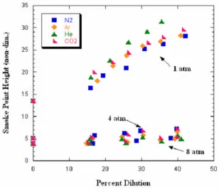
Figure 4.2: Smoke point height as a function of percent dilution for a diluted ethylene flame at 1, 4, and 8 atmospheres... 46

Figure 4.3: Volumetric fuel flow rate versus diluent flow rate at (a) 1, (b) 4, and (c) 8 atmospheres with curve fits for CO2 and He ... 48

Figure 4.4: Volumetric fuel flow as a function of volumetric diluent flow for a plug and parabolic exit velocity profile along with previous researcher's findings ... 50

Figure 4.5: Volumetric fuel flow and smoke point as a function of fuel to air velocity ratio for undiluted ethylene in two different burner configuratio ns ... 52

Figure 5.1:Watec 902 Ultimate monochrome CCD camera with ND filter and color filter wheel... 57

Figure 5.2: Black body calibrator ... 58

Figure 5.3: Pure ethylene soot surface temperature profiles as a function of pressure ... 59

Figure 5.4: Soot surface temperature profiles of ethylene flames diluted 40% by volume .... 61

Figure 5.5: Maximum soot surface temperatures for (a) undiluted ethylene and (b) ethylene with 40% dilution... 64

Figure 5.6: Soot volume fraction and soot surface temperatures as a function of pressure for undiluted, constant fuel mass flux ethylene flames ... 66

Figure 5.7: Measured soot surface temperature with radiative losses represented ... 68

Figure 6.1: Final quartz microprobe design ... 76

Figure 6.2: C2H2 concentration in (a) helium and (b) carbon dioxide diluted flames ... 81

Figure 6.4: C6H6 concentration for (a) helium and (b) carbon dioxide diluted flames... 86

Figure 7.1: Extinction measurement schematic ... 96

Figure 7.2: Comparison of soot volume fraction measureme nts at 1 atmosphere ... 99

(11)

Figure 7.5: Soot volume fraction (a), in ppm, and temperature (b), in Kelvin, profiles for He (left) and CO2 (right) diluted flames at 2 atmospheres ... 104

Figure 7.6: Extinction measurements of soot volume fraction as a function of radial position at 2 atmospheres in diluted flames ... 106 Figure 7.7: Soot volume fraction (a), in ppm, and temperature (b), in Kelvin, profiles for He (left) and CO2 (right) diluted flames at 4 atmospheres ... 108

Figure 7.8: Extinction measurements of soot volume fraction as a function of radial position at 4 atmospheres in diluted flames ... 110 Figure 7.9: Soot volume fraction (a), in ppm, and temperature (b), in Kelvin, profiles for He (left) and CO2 (right) diluted flames at 8 atmospheres ... 111

(12)

1 Introduction

In a society that depends heavily of a depleting supply of non-renewable fossil fuels

in order to make energy for heat and work, eliminating inefficiencies from combustion

devices that run on these fossil fuels is becoming more and more critical. It is known that

diffusion-flame-driven devices are much more fuel efficient than premixed- flame-driven

devices, but with this increased efficiency comes the disadvantage of more pollutant

formation, particularly soot and NOx. Since these diffusion-flame-driven devices can

provide a more efficient means to meet energy demands, research efforts should be focused

on reducing or eliminating the pollutant formation from these combustion devices while

maintaining fuel efficiency. Of these pollutants formed through the combustion process,

particulate matter is of greatest concern. Particulate matter, such as soot, is a risk not only to

the environment, but also to human health. Soot has been proven to be a carcinogen and a

mutagen as well as causing more long-term illnesses such as chronic bronchitis (Sydbom et

al., 2001; Comstock et al., 1998; Morgan et al., 1997; Scheepers et al., 1992). Because of

these environmental and human health effects soot entails, the Environmental Protection

Agency (EPA) continues to stringently monitor and regulate particulate emissions from all

sources, both mobile and stationary. Heavy-duty Diesel engines continue to come under

strict regulations for emissions from the EPA, and Diesel engine manufacturers find it

(13)

the interactions between combustion chemistry, transport, and fluid mecha nics, but a

complete understanding of these interactions is not known by the combustion community at

this time. The majority of the research conducted currently is accomplished at atmospheric

conditions and not at elevated pressures where these devices operate. The lack of research at

elevated pressures is due mostly to cost, time, and safety issues. Despite these drawbacks,

this research is necessary to increase the pool of knowledge in order to reduce or eliminate

soot production from these diffusion- flame-driven devices.

The current research used ethylene and methane, both pure and diluted (individually

with helium, nitrogen, argon and carbon dioxide) from 1 to 16 atmospheres to investigate

smoke point height, fuel exit velocity profile effects, soot surface temperatures, hydrocarbon

species concentrations, and soot volume fraction. Each of these investigations was

conducted in order to gain the necessary information to evaluate the hydrogen absorption

carbon addition (HACA) soot growth mechanism at elevated pressures. This soot growth

mechanism is widely accepted in the combustion community, but has not been thoroughly

investigated at elevated pressures where most practical combustion devices operate. Each

phase of the experiments is documented within this paper and as the experimental apparatus

changes for each experiment is it noted. In most cases, except where noted, the air to fuel

velocity ratio remains at unity and the flames are kept at their smoke point. By limiting these

experiments to velocity- matched and smoke point conditions, this research eliminates

possible causes for discrepancies from laboratory to laboratory and makes the data

reproducible and easier to compare and contrast to the research of other investigations.

(14)

reason for that particular phase of the experiment, each individual experimental apparatus,

the results and discussion obtained from each phase, and finally the conclusions that are

apparent from each phase as well as the overall conclusions reached from the entire

investigation.

1.1 Soot Formation and Growth

Recent research has focused on a better understanding of soot growth and formation.

Investigators have determined that a better understanding of chemical kinetics transport, and

fluid mechanics would greatly increase the combustion community’s understanding of soot

formation. Although some understanding exists for the chemical kinetics, transport, and

fluid mechanics, the interactions between these three functions are also of great interest and

not very well understood at all, and it has been determined that, as a community, our research

efforts should be focused on these interactions (Frenklach, 2002; Richter & Howard, 2000).

Diffusion flames and premixed flames have very contrasting qualities that must be

understood prior to being able to conduct research. Diffusion flames, as stated earlier, will

produce more soot than premixed flames. This is due to the fundamental controlling

mechanisms present in diffusion flames. In diffusion flames, the fuel and the oxidizer are

stored separately and do not come into contact with one another until they reach the primary

reaction zone. The fuel and oxidizer then diffuse into the reaction zone due to the

(15)

oxidizer present and then the fuel and oxidizer enter the reaction zone together. Furthermore,

in the premixed flame soot is created when the oxidizer is absent, as it is responsible for the

converting of hydrocarbons into carbon monoxide and diatomic hydrogen. It has been shown

by Wagner (1981) experimentally that if the ratio of carbon to oxygen atoms for the flame is

greater than 0.5, the premixed flame will produce soot. The converse of Wagner’s findings

also holds true such that soot will not be produced if a non-soot- yielding ratio of carbon to

oxygen atoms is maintained in the mixture region. Controlling and maintaining the ratio of

carbon to oxygen atoms in the mixing region in a diffusion flame is typically not possible,

which makes an environment more suitable for soot production.

Whether dealing with a diffusion or premixed flame, soot formation begins in the

same manner, in the preheat zone. It is in the preheat zone that the large molecules

decompose into smaller hydrocarbon pieces because of increases in temperature that occur in

this zone. Soot precursors are formed because of this pyrolysis and take the form of

acetylene (C2H2). Hydrocarbon fuels that have a low propensity to form soot, such as

methane (CH4), have low soot production because they have a more difficult path to

thermally decompose into acetylene. However, more complex hydrocarbons, such as

ethylene (C2H4), have a much easier path to thermally decompose into acetylene and thus

have a much higher propensity to form soot. After the precursors to soot are created, the

acetylene molecules combine in groups of three to form benzene rings (C6H6). Several of

these benzene rings then combine to form polycyclic aromatic hydrocarbons, typically

referred to as PAHs. Then the process of polymerization begins and the rings of benzene

(16)

the rings become unsaturated. As this process continues, the carbon to hydrogen atom ratio

increases and causes the rings to group together forming the soot particle, often called a soot

spherule. These soot spherules continue to grow in size up to roughly 30 to 50 nm in

diameter. Just one of the many things researchers do not understand about soot formation is

why the soot spherule’s growth discontinues at this range of diameters. However, after the

soot spherules reach this diameter range, they begin to join together to form agglomerates,

which end up containing hundreds to thousands of soot spherules. Then these agglomerates

join together to form clusters, which result in soot particles (Figure 1.1). These soot particles

have an estimated empirical formula of C8H.

Figure 1.1: Soot spherules forming agglomerates (Gaydon & Wolfhard, 1970)

(17)

growth. The visibly yellow portion of a flame (a candle for instance) is the soot

incandescence. If the soot in this soot incandescence region is oxidized prior to diffusing

across the flame front, the flame with cease to emit visible smoke. This is how the

distinction between soot and smoke becomes apparent. Any carbon that leaves the flame is

smoke, but any carbon that stays within the flame and is oxidized, forming CO or CO2, is

considered soot. Early investigations by Schalla and co-workers (1955) looked at the

difference between smoke and soot production in diffusion flames at atmospheric and

elevated pressures.

1.2 Effects of Elevated Pressure on Soot Formation

A very well known and well researched aspect of diffusion- flame-driven devices is

that the soot production increases, while soot oxidation decreases, with increasing pressure

(Flower & Bowman, 1986). However, as mentioned previously, experimental research at

elevated pressures is limited because of its timely, costly, and dangerous nature. More recent

research is moving towards experimental research at elevated pressures, such as the current

research, in order to better understand pollutant formation from combustion devices at their

normal operating conditions. Researchers, although they do not fully understand why, agree

that increasing the pressure surrounding a diffusion flame increases the reaction rates and the

diffusion coefficient of the flame, thus leading to increased soot production. Other

researchers, who have focused on spray combustion and premixed- flame-driven combustion,

have seen increases in soot production in these devices when the environment surrounding

(18)

Kadota et al., 1977; Miller & Maahs, 1977; Millberg, 1959; Fischer & Moss, 1998;

Heidermann et al., 1999).

Previous research by McCrain and Roberts (2005), conducted in a similar burner and

vessel configuration as the current research at elevated pressures, was able to measure the

effects of elevating pressure. Working with laminar diffusion flames, they were able to

measure the soot volume fraction, fv. The current work also investigates the soot volume

fraction in laminar diffusion flames at elevated pressures, but uses a different technique,

described below in detail in §1.7, from McCrain and Roberts (2005) who used laser induced

incandescence (LII) and extinction measurements.

Increasing the pressure inside the vessel has a few impacts on the flame. With the

reaction rates increasing in proportion to the pressure and the diffusion rates increasing as the

gradients become steeper, the flame becomes thinner, less stable, and shorter. These changes

to the flame were expected, and similar findings involving pressure effects on flames were

reported by Miller and Maahs (1977). They showed that hydrodynamics disrupt the flame

and make it more sensitive to extinction because the diffusion of reactants cannot occur

quickly enough to restore the flame.

1.3 Smoke Point

The smoke point of a flame has been recognized in the combustion community, for

many years, as a fundamental measure of a fuel’s propensity to soot. Smoke point has been

(19)

1.2, it is possible to see the distinct difference between two flames at and just slightly above

their smoke points. The flame on the left has a volumetric fuel flow rate of 76 sccm and an

air co-flow rate of 16.6 SLPM. The flame on the right, which is slightly above its smoke

point, has a volumetric fuel flow rate of 98 sccm and an air co- flow rate of 21.7 SPLM. In

each flame the air to fuel velocity ratio is unity. In the flame on the right, which is just above

its smoke point, it is possible to see visible smoke from the tip and feathering of the flame

(called wings) near the tip which is a sign of a flame reaching and exceeding its smoke point.

Figure 1.2: Undiluted ethylene flame at 2 atm at smoke point (left) and just above smoke point (right)

The smoke point can also be described as the position of the flame where the soot production

and soot oxidation directly offset one another. It should be noted that the current research

was conducted with gaseous fuels rather than liquid fuels. There is limited experimental

research published regarding the smoke point of gaseous fuels, and even fewer publications

exist that focused on smoke points of diluted fuels or the effects of pressure (Dai & Faeth,

(20)

Glassman & Yaccarino, 1981; Schalla et al., 1954). Furthermore, only slightly more research

on smoke points, using numerical simulation has been conducted and published (Guo et al.,

2002; Delichatsios, 1994; Kent, 1986). The work of Schalla and co-workers (1955),

mentioned previously, examined the smoke and soot production in diffusion flames and

recorded flame heights at smoke points for ethylene and ethane flames from 0.5 to 20

atmospheres. They worked with not only wick- fed liquid fuels but also with gaseous fuels.

Although they had no way of metering and recording the fuel flow rates, they were able to

measure the flame’s height at its smoke point. They reported that the flame height decreased,

nearly linearly, with the increasing pressure for gaseous fuels. At the time they believed this

effect to be caused by diffusion rates and the rate of mixing of the fuel and air. Dai and

Faeth (2000) investigated laminar diffusion flames and the air to fuel velocity ratios effects at

sub-atmospheric pressures to find that the flame’s height at its smoke point is twice as long

as a soot- free (blue) flame under the same conditions. Urban and co-workers (2000) also

tested with laminar diffusion flames, but in microgravity conditions, and reported that

contrary to normal gravity conditions, the smoke point occurred in two configurations:

closed-tip flames with soot emissions along the flame axis and open-tip flames with soot

emissions from an annular ring about the flame axis.

In the current experimental research diffusion flames are investigated and the

luminous flame height and mass flow rates were recorded at the smoke point of pure and

diluted flames. Since the current research sought to investigate combustion devices at

(21)

atmospheric conditions, but also at elevated pressures up to 8 atmospheres for ethylene and

up to 16 atmospheres for methane.

1.4 Fuel Exit Velocity Profile and Dilution Effects

The investigation into the effects of the fuel exit velocity profile was not initially

anticipated as a phase of this research. However, after the smoke point data was collected

and compared to that of previous researchers, it was necessary to investigate the fuel exit

velocity profile and the effects of different inert diluents in order to explain the discrepancy

between the current experiment and the experiments of previous researchers.

1.4.1 Diluent and Dilution

Previous researchers have investigated the effects of dilution on smoke point in laminar

diffusion flames at atmospheric pressures. McLintock (1968) investigated the effects on

smoke point and sooting tendencies by adding inert diluent to either the fuel or oxidizer

stream. It was found that dramatic differences in the smoke point existed when using

different diluents, with carbon dioxide (CO2) having a very strong ability to suppress soot

production and helium (He) having a very weak to no ability to suppress soot production.

Both nitrogen (N2) and argon (Ar) fell in between CO2 and He, but much closer to He, in

their ability to suppress soot formation. For McLintock’s experiments the air co-flow

velocity was held constant with an initial fuel-to-air velocity ratio of approximately 1.4,

which increased with dilution level. At the initial fuel-to-air velocity ratio, McLintock found

(22)

plotting the volumetric fuel flow rate at the smoke point versus the volumetric diluent flow

rate.

Glassman and co-workers (1998, 1980) found similar trends when using these

diluents in a highly over-ventilated environment (with unreported, but presumed constant, air

co-flow velocity), but showed CO2 having an even stronger soot suppression effect than

McLintock (1968) had reported. Glassman and co-workers plotted the volumetric fuel flow

rate versus the volumetric diluent rate and found a slope of 1.10 for CO2 and a slope of 0.2

for He. Although the results of Glassman and McLintock differ slightly, the observation that

CO2 is much more efficient than He at suppressing soot is consistent. Since the findings of

the current experiments differ, showing very little difference in soot suppression at the smoke

point height using CO2 versus He, from those of previous investigations, this experiment to

investigate fuel exit velocity profiles and dilution was added as a phase in the research.

Previous investigations into dilution of a fuel or oxidizer stream have shown that

there is both a thermal effect, scaling with molar heat capacity of a diluent, and a dilution

effect, scaling with the molecular and thermal diffusivities of a diluent (Guo et al., 2000,

2004). Many researchers have used the same diluents for investigation as the ones chosen for

the current experiments: He, Ar, N2, and CO2. The use of these diluents, to investigate the

effects of diluent addition to ethylene and methane flames, makes it possible to cover a broad

(23)

Table 1.1: Transport properties of the four diluents at 20 degrees Celsius

Helium Carbon

Dioxide

Argon Nitrogen

Specific Heat Capactiy

(J/kg C) 5193 846 520 1042

Kinematic Viscosity

(cm2/s) 1.15 0.08 0.12 0.15

Thermal Diffusivity

(cm2/s) 1.59 0.10 0.18 0.19

Binary Diffusion Coefficient into N2 (cm

2

/s) 0.71 0.16 0.20 0.22

With the addition of any of these diluents, to a fuel or oxidizer stream, there is a change in

the viscosity and therefore the shear layer growth and entrainment is effected. Therefore, it

is expected that He should have more of an effect on entrainment and mixing than CO2, with

N2 and Ar falling between them. Table 1.1 shows the kinematic viscosities, thermal and

molecular diffusivities, and the specific heats of the four diluents (Kanury, 1994). From the

values in this table it is made clear the property differences between He and CO2, such that

they differ by a factor of 15 in both kinematic and thermal diffusivity but only a factor of 5 in

molecular diffusivity. This provides a unique effect on the ethylene when either of the two

diluents is used.

The transport and thermal effects on soot suppression by a given diluent is important

to consider, but the possible chemical effects must also be considered. Glassman (1998) and

Schug (1980) both postulated that there were chemical effects with the addition of CO2 in

addition to the thermal and transport effects. Later, in 2001, Liu and co-workers showed

computationally that these chemical effects do suppress soot formation by reducing both the

(24)

converting CO2, by hydrogen atom, to carbon monoxide and hydroxyl prompts the oxidation

of soot precursors in the formation region. They further found that not only does the addition

of CO2 to the fuel stream reduce soot formation, but this addition also reduces NOx formation

through suppression of the temperature.

1.4.2 Exit Velocity Profiles

As stated previously, the initial intent of this particular experiment was not to study

the effects of fuel exit velocity profile on smoke point, but rather to identify potential reasons

for the discrepancies observed with dilution compared with the findings of previous

researchers.

Faeth and co-workers identified and aerodynamic means of affecting the diffusion

flame by reducing the shear layer effects between the fuel and the air co-flow (Lin & Faeth,

1996; Dai & Faeth, 2000). They were able to show that the closer to unity the fuel-to-air

velocity ratio falls, the effect of the shear layer becomes smaller and nearly negligible. Prior

to Faeth’s work, Roper and co-workers (1977) reported that smoke point was insensitive to

the fuel to air velocity ratio as long as the flame was highly over-ventilated. This led some

researchers to conclude that for gaseous fuel laminar flames, the smoke point and soot

concentrations are dominated by buoyancy and molecular diffusion, and are insensitive to

viscous effects. Ultimately, this was proven to not be the case.

Faeth and co-workers (1996, 2000) showed the velocity ratio to have great effect on

determining smoke point characteristics of a particular fuel. The found that in these laminar

(25)

substantially increasing the air co-flow rates. For the majority of the current research, and

research conducted by Berry and Roberts (2006), a plug flow fuel exit velocity profile and a

fuel to air velocity ratio of unity was employed. As stated above the plug flow fuel exit

velocity profile was necessary to eliminate oscillations in the flames as pressure within the

vessel was increased, and the velocity ratio of unity was used to minimize shear layer effects.

In contrast, many of the researchers completing similar experiments have used parabolic fuel

exit velocity profiles and a plug flow air exit velocity. In most of the experiments of other

researchers, the velocity matching between fuel and air, if it ever occurred, only occurred at

the initial undiluted conditions. Therefore, as diluent was added to their fuel stream the fuel

exit velocity increased, maintaining the over-ventilated status, but the air co-flow velocity

remained constant.

When the velocities are not matched, shear layer and entrainment scales with the

viscosity and therefore the diluent choice becomes important. Smooke (2005) showed,

experimentally and computationally, the importance of the velocity ratio in diffusion flames.

Their investigation was performed in a velocity matched parabolic velocity profile flame at

atmospheric conditions.

The Froude number (G) determines whether the flame is momentum or buoyancy

dominated, as it is a dimensionless ratio between inertial and gravity forces. The Froude

number was calculated for the current investigation using the atmospheric, undiluted ethylene

flame and had a value equal to 0.21, and thus it is buoyancy controlled. With increasing

pressure causes a decrease in Froude number, thus all of the flames in this investigation are

(26)

1.5 Soot Surface Temperature

In order to reach the overall goal of investigating the accuracy of the HACA

mechanism at elevated pressures it was necessary to complete soot surface temperature

measurements from the flames at and above atmospheric pressure. These measurements are

necessary to understand the structure of the flame, as temperature can affect the

concentrations of species among other characteristics of the flames. Experiments by

previous researchers have focused on soot surface temperature measurements but only at

atmospheric pressure conditions (Hall & Bonczyk, 1990; Cignoli et al., 2001; Xu et al.,

2003). More recent research, conducted by Thomson and co-workers (2005) has focused on

these measurements with elevating pressure and has shown an overall decrease in soot

surface temperature as pressure increases. Also, they observed that the temperature increased

axially from the base to the tip of the flame. Throughout the current experiment the same

trends in soot surface temperatures were recognized; however, a major difference between

the current experiment and those of previous researchers is that the current measurements

were taken at the flame’s smoke point.

1.6 Hydrocarbon Species Concentrations

Yet another essential piece of information that was required to analyze the HACA

mechanism at elevated pressures was species concentrations. This experiment focused on

hydrocarbon species only, but future experiments to be conducted in the near future by

(27)

concentrations were measured by extracting samples from ethylene flames and analyzing

them with gas chromatography with a flame ionization detector (GC-FID). Unlike the

previous experiments discussed thus far in the current investigation, the flame for this

experiment were not at their smoke point; however, they were velocity matched such that the

reactant flow (fuel plus diluent) velocity was matched with the air co- flow velocity. The

samples were extracted through a probe and in order to avoid clogging of the probe, it was

necessary to use very heavily diluted flames, 80% by volume. However, these flames

remained highly over-ventilated and buoyancy dominated at all pressure conditions.

Hydrocarbon species have been investigated by many researchers in the last ten to

fifteen years both computationally (Smooke et al., 1999; McEnally et al., 2000) and

experimentally (McEnally & Pfefferle, 1999; Kim et al., 2004 & 2008). However, excluding

the most recent work by Kim and co-workers (2008), these measurements have been

accomplished at atmospheric pressures. Also, in each of the investigations by previous

researchers the species concentration measurements have been taken along the centerline of

the flame. The current research extracted samples not only along the centerline, but also

along the surface of the flame. Nearly all of the samples collected were within the blue

(soot- free) region of the flame with only a few samples reaching in to the soot incandescence

(yellow) region of the flame.

1.7 Soot Volume Fraction and Pyrometry

Soot mass yield is one characteristic that can be useful in determining the parameters

(28)

flame. There are several experimental methods that can be incorporated to measure soot

volume fraction such as LII, laser extinction, and pyrometry, to name a few. Of all the

research that has been conducted over the years pertaining to soot volume fraction, some of

which has been conducted at elevated pressures, it is clear that the researchers are in

agreement that as pressure increasing the soot volume fraction also increases.

One of the first investigations into soot volume fraction at elevated pressures was

conducted by Flower and Bowman (1986). They were able to measure soot volume fraction

from 1 to 10 at atmospheres, showing experimentally that as the pressure increases the rates

of soot production and growth also increase. Flower and Bowman collected line integrated

soot volume fraction measurements using laser scattering techniques, but unfortunately these

measurements to not provide results that are spatially or temporally resolved.

As mentioned previously, more recent experiments have been conducted, with a

similar burner and pressure vessel to that used in the current investigation, to investigate not

only soot volume fraction, but the effects elevated pressure has on soot volume fraction.

McCrain and Roberts (2005) used a diffusion flame, with undiluted methane or ethylene, to

measure integrated and peak soot volume fraction. The technique chosen for these

measurements were LII and extinction. They found that integrated fv of methane scales

approximately as P1.0, and for ethylene approximately as P1.2. They also found that peak fv

for methane and ethylene scales approximately as P1.2 and P1.7, respectively. This research

was conducted in the same pressure vessel as the current research, and the measurements

(29)

ethylene. Their work was unique in the fact that no other researchers had ever measured

peak soot volume fraction.

1.7.1 Refractive Index of Soot

The refractive index of soot has been widely disputed over the past half of a century,

especially in laboratory scale experiments. In 1969, Dalzell and Sarofim published a journal

article describing the best value to be used for the index of refraction for soot, 1.57-i0.56.

This value became widely accepted and many researchers still continue to use this particular

index of refraction. However, more recent investigations into the refractive index of soot

have led researchers to choose their value to be more specific to their particular laboratory

set-up. Chang and Charalampopoulos (1990) experimentally showed that there is a

wavelength dependence for the soot refractive index. They combined classical and dynamic

light scattering measurements and the Kramers-Kronig relations to express refractive index

of soot for specific wavelengths, thus making the decision for the refractive index assumption

specific to experimental apparatus. They performed these measurements and calculations for

a range of wavelengths and then were able to determine an equation (Eq. 1.1) that can be

used to calculate the refractive index of soot for a given experiment.

(30)

For the pyrometry and laser extinction methods used in the current experiments, using the

above equation, the refractive index of soot was determined to be 1.75- i0.57.

1.7.2 Two Wavelength Emission Technique

This technique for measuring the temperature profile and soot volume fraction along

the centerline of the flame has been shown to be rather accurate (De Iuliis et al., 1998;

Cignoli et al., 2001; Boiarciuc et al., 2006). Boiarcius (2006) conducted measurements of

soot volume fraction and particle size estimates using both the two color emission method

and the classic method of LII and found that the two color emission technique is just as

accurate, but requires less time and equipment. Cignoli and co-workers (2001) extended on

the two-color pyrometry (discussed in §1.5) technique and used mathematical equations to

solve for the soot volume fraction based on the emissions of the flame, emission from a

known source (a tungsten lamp), the temperature profile, and the spectral properties of soot

to measure the soot volume fraction in flames. Although the current experiment employs a

black body calibrator to create a temperature calibration for the flame’s profile, the same

equations used by Cignoli et al. (2001) and De Iuliis et al. (1998) was used to determine soot

volume fraction for the flames in the current experiment. As stated previously (§1.5), the

two-color pyrometry yielded a temperature profile of each flame. The same fourth-order

equation, based on Planck’s equation, was used, but a new calibration was necessary

according to the needed camera settings for these measurements in order to generate a

temperature profile. Then, using that temperature profile, and updating and adding to the

(31)

                    ₋ − − = s L L S abs v T T c E E L

f ln 1 0.99 *exp 1 1

λ

λ λ l

(1.2)

where, labs is the natural length of absorption at a given wavelength with respect to soot

spectral properties (calculated), L is the width of the flame under consideration (measured),

ES? is the integration process over the optical path (measured), EL? is the intensity of the

calibrated lamp emission (given), c is Planck’s constant (given), ? is the wavelength of the

filter (in µm), TL is the lamp or black body calibrator temperature (measured), and TS is the

soot temperature determined from the image ratio (measured), the soot volume fraction is

calculated.

1.7.3 Laser Extinction and Tomographic Inversion Technique

The laser extinction method is the same method employed by McCrain and Roberts

(2005) to yield ave rage soot volume fraction, and used by many other researchers. This

method uses a helium- neon (HeNe) laser beam and passes the beam through the flame.

When the laser beam passes through the flame the energy is removed by molecules or

particles, such as soot. The soot particles scatter and absorb the laser energy and the beam

becomes attenuated. Another beam is passed directly above the flame, but parallel to the

beam passing through the flame to yield an unattenuated beam. The ratio of the attenuated

and unattenuated beam can be used to calculate average soot volume fraction. D’Alessio and

(32)

Rayleigh scattering regime (where d<<?) to solve for average soot volume fraction using the

following equation:

{

(

1 )

/(

2 )

}

Im

)

/

ln(

6

2 2

,



−

+











=

m

I

L

f

_sv_ave o

π

λ

(1.3)

where in this case, ?=632 nm (He-Ne laser beam), L is the path length, I is the attenuated

intensity, I0 is the unattenuated intensity, and m is the refractive index of soot. As stated

above, in §1.7.1, the value used in this particular experiment for the refractive index of soot

is 1.75-i0.57.

Once the extinction measurement s were completed, these values for average soot

volume fraction for each flame is used, along with a tomographic inversion technique, to

solve for the soot distribution at a given height in the flame. Other researchers have

previously used this technique to investigate soot volume fraction and distribution at

(33)

2 General Experimental Apparatus

For the majority of the experiments throughout this investigation the co-flow burner

and the pressure vessel remained the same. However, at times during certain experiments the

co-flow burner was modified, and in one experiment a second co- flow burner was utilized.

This section details the co- flow burner, pressure vessel, chimney, and ignition most often

used throughout this investigation. In the following chapters, when applicable, changes or

modifications to the burner or chimney that were necessary for each particular experiment

are documented.

2.1 Co-Flow Diffusion Flame Burner and Chimney

The burner, modeled as the classic over- ventilated Burke-Schumann (1928) laminar

diffusion flame, used for this investigation has a fuel tube diameter of 4.5 mm and an air

(34)

Figure 2.1: Co-flow diffusion flame burne r cup

In order to minimize pressure fluctuation effects on the fuel flow rate, stainless steel wool

(0000 gage) was inserted into the fuel tube. This created an isolated pressure drop and a

uniform, also referred to as plug or top-hat, exit velocity profile. The steel wool was

necessary for measurements made at elevated pressure, within the vessel, to isolate the fuel

flow rate from small fluctuations that in turn would cause large changes in the fuel flow rate.

As discussed previously, using a plug flow exit velocity profile did cause some discrepancies

between the results of this investigation and the results of others. However, as explained

later in chapter 3, these discrepancies were studied and it was possible to show that the

current experiments were in agreement with other researcher’s experimental results when a

(35)

compare atmospheric as well as elevated pressure results, and since the elevated pressure

conditions required flow straightening of the fuel flow, the flow straightener in the fuel tube

was necessary for the majority of the experiments, resulting in a plug fuel exit velocity

profile. It should also be noted that the fuel and the diluent entered the burner through the

fuel tube; however, they were introduced well in advance of the fuel exit plane and therefore

were considered fully mixed.

The air co-flow portion of the burner had a combination of hollow glass spheres and

ceramic honeycomb to instill uniform exit velocity profile. A quartz chimney was also

utilized with the co- flow burner at both atmospheric and elevated pressure conditions. This

chimney had an outside diameter of 71 mm, a 3 mm wall thickness, and a 40 cm overall

height. This chimney, though slight modifications were necessary from experiment to

experiment throughout this investigation (describe in detail in future sections), was necessary

to combat air perturbations within the pressure vessel, caused by the geometry of the vessel.

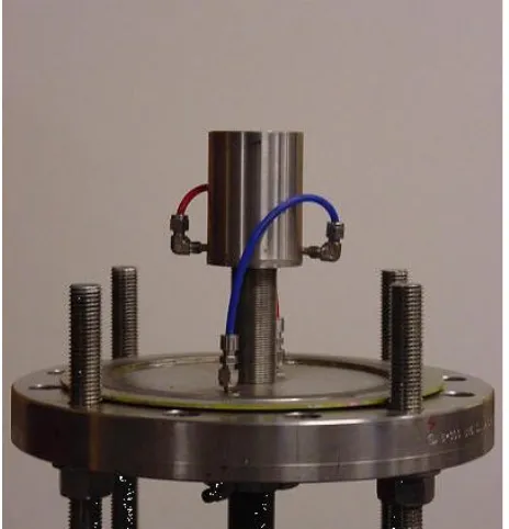
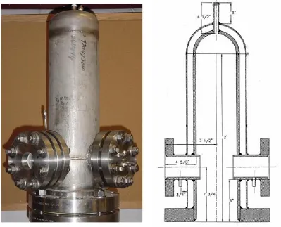
2.2 Pressure Vessel and Ignition System

The vessel in which the co- flow burner is housed is a water cooled pressure vessel

that is capable of continuous operation up to 30 atmospheres, although for this investigation

it was not used at any greater pressure than 16 atmospheres. It was designed and originally

built by Li (2001), shown in Figure 2.2. The vessel is one meter tall and has four flanges

extended beyond its circular body. In three of these flanges there are glass windows,

constructed of BK-7 (diameter of 7.6 and thickness of 2.5 cm), that allow for optical viewing

(36)

holes for intrusive diagnostics. Because of the fuels used, and their sooting tendencies, the

vessel has air ports on two of the windows to purge the area and prevent accumulation, of

condensation and soot, on the window surface and thus allowing optical access. The co-flow

burner housed inside the vessel is

Figure 2.2: High pressure vessel with dimensions

capable of vertical translation, allowing for optical access to all portions of the flame. The

(37)

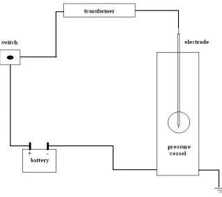
resistance to ground spark was not reached until it came into contact with the stainless steel

fuel tube, several layers of electrical tape were applied to the outside of the ceramic.

The electrode was place inside the exhaust port of the pressure vessel and lowed

through the open end of the quartz chimney, and then was place 3 to 5 mm from the fuel

tube. Since the electrode passed through the exhaust port it was removed once ignition had

occurred so the exhaust value could be replace on the exhaust port to meter the pressure in

the vessel during experiments. As diagramed in Figure 2.3, the portion of the exposed

copper wire that was outside of the pressure vessel was attached to an electrical cable that ran

to a low-to-high voltage transformer, which was powered by a 12 volt deep cycle marine

battery.

(38)

A toggle switch between the battery and the transformer provided an electrical arc inside the

pressure vessel from the copper wire to the fuel tube lip. This provided a very strong spark

for the ignition of the flame within the vessel.

2.3 Pressure Metering

Elevating the pressure within the vessel is time consuming and very sensitive. The

pressure is built in the vessel based on a simple concept of mass in versus mass out, such that

the reactant and air come through the burner into the vessel and then the amount of products

that are released from the vessel controls the pressure within the vessel. The air provided for

combustion comes from compressed cylinders to ensure enough back pressure to sustain the

pressure inside the vessel, the air is also ensured to by dry. A needle valve is attached to the

exhaust port of the vessel and by opening and closing the needle valve the pressure can be

metered. However, if at any time the needle valve closes completely the flame inside the

vessel will be extinguished. The pressure inside the vessel is displayed on an external gauge

and has a range of 0 to 1000 psig. The mass flux of co- flowing air is increased, while the

needle valve is closed slowly to build pressure. It proves to be a taxing chore to maintain a

velocity matched fuel to air ratio and building pressure within the vessel, while maintaining a

flame that is not providing too much soot to the inside of the vessel. Window air is kept

flowing (to prevent soot and condensation build-up on the windows), but with a very

(39)

2.4 Fuel Flow Metering

In the base of the pressure vessel two ports exist, one for fuel and diluent inlet and the

other for air co- flow inlet. Stainless steel fittings and plastic fuel lines carry the fuel, diluent,

and air to the burner cup from the base of the vessel. On the outside of the pressure vessel,

stainless steel fittings attach to stainless steel braided lines to carry the fuel, diluent, and air

from the compressed cylinders, to the flow meters, and then on to the pressure vessel. As

mentioned previously, two ports do exist on two of the optical flanges to provide air to the

remove debris and condensation from the windows.

All of the air provided to the pressure vessel (both to the burner cup and to the

window air) ran from the compressed cylinders to separate TeleDyne Hastings mass flow

meters (Model 201). Each of these flow meters was calibrated with nitrogen for a range of 0

to 100 standard liters per minute (SLPM).

As for the fuel and the diluent, each was carried to individual TeleDyne Hastings

mass flow meters (Model 200) that were calibrated with nitrogen for much slower flow rates,

1 to 1000 standard cubic centimeters (sccm). Each of the fuels (methane or ethylene) and

diluents (helium, nitrogen, argon, or carbon dioxide) used were at least 99% pure and each

mass flow meter was calibrated for the individual use of these gases.

Each of the four TeleDyne Hastings mass flow meters was powered by the same

TeleDyne Hastings power supply (Model 40). This power supply not only provided power,

but also provided a digital read-out of the flow rates for each meter. Since each of the flow

meters was calibrated using nitrogen, it was necessary to input a correction factor, into the

(40)

factors and are provided by the manufacturer for air, ethylene, methane, argon, helium, and

(41)

3 Smoke Point in Pure Ethylene and Methane Flames

3.1 Background

Although a large portion of the smoke point height measurements was accomplished

while the author was seeking the degree of Master of Science, all of these measurements

were repeated while the author was seeking the current degree of Doctor of Philosophy, and

are essential to the fundamental understanding of the more recent research and therefore this

experiment and its findings are included in this paper.

As mentioned previously, the smoke point of a fuel specific flame is a measure of the

fuel’s propensity to soot. It is the point at which the soot production and oxidation are

directly offset and thus no visible smoke is emitted from the flame. For this experiment, pure

ethylene and methane flames were tested up to 8 and 16 atmospheres, respectively to

measure the smoke point height of each flame.

3.2 Experimental Apparatus

The most basic form of the current co- flow burner set- up was utilized for these smoke

point height measurements. The burner, as stated previously, had a fuel tube diameter of 4.5

millimeters, a co-flow diameter of 65 millimeters, and a solid quartz chimney with an inside

diameter of 65 millimeters. The fuel exit velocity profile, with stainless steel placed in the

fuel tube, was plug.

Methane was chosen because it can be used to represent natural gas, which is

(42)

soot. Ethylene was chosen as a representation of a complex hydrocarbon with a very high

propensity to soot. A more commonly used fuel, propane, was considered for the

experiments, but since propane has such a low saturation pressure at room temperature

elevated pressure testing would have resulted in a liquid form of propane rather than a

gaseous form.

The methane testing was completed over the pressure range of 2 to 16 atmospheres,

while the ethylene pressure testing ranged from 1 to 8 atmospheres. Obtaining a pure

laminar, steady, methane flame at atmospheric proved to be impossible in the current burner.

However, other researchers have experienced the same problem with methane diffusion

flames at atmospheric conditions (Kent, 1986). Each of the flames was tested at its smoke

point and with fuel to air velocity ratios equal to unity.

To determine the smoke point height of each flame an iterative approach was used

to adjust the fuel flow rate and air co-flow rate to unsure that the velocity ratio remained at

unity. Fuel was increased until the flame emitted visible smoke and then the air co- flow was

increased to the velocity matched ratio. If the visible smoke from the flame then ceased,

more fuel was added to get to a smoking flame, and then the air increased, continuing this

process until the velocity matched fuel to air ratio smoke point height of the flame was

obtained. As the experiments were repeated several times, the iterative process improved to

where roughly three iterations were required to obtain each smoke point height. Once the

smoke point was reached, an image of the flame was taken with a digital camera and later

(43)

As mentioned above, the current experiments were completed for the visible smoke

point, and therefore the smoke point heights reported within should be understood to be

luminous smoke point heights and not stoichiometric contour height measurements, which

other researchers have investigated previously (Newman et al., 2004).

3.3 Results and Discussion

In order to determine the effects pressure has on the overall kinetics of the soot

inception and oxidation portions of the soot formation process, smoke point height

measurements were made. These smoke point heights were measured and then

non-dimensionalized, by the fuel tube diameter (4.5 mm), for ease of comparison of results.

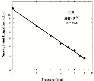
Figure 3.1 shows the non-dimensionalized smoke point height of ethylene as a function of

(44)

(45)

The data in each of these figures is plotted in log- log space, and in this configuration the data

fit to a power law where the smoke point height scales as a function of pressure to the -0.69

for ethylene and -0.29 for methane. In each case the smoke point height varied from the

results of Schalla and co-workers (1954) in which they found the smoke point height to

decrease nearly linearly with increasing pressure. These findings were the first that would

later prompt the fuel exit velocity profile experiments (discussed in Chapter 4), as it was

believed that these discrepancies were due to the plug fuel velocity exit profile used for this

experiment.

The volumetric fuel flow rate (FFV) was also plotted as a function of pressure, for

both ethylene (Figure 3.3) and methane (Figure 3.4), in order to determine if a functional

dependence of FFV on pressure exists at the smoke point. In both instances, pure ethylene

and pure methane, the best trend fit is available in log- linear space, yielding a logarithmic

dependence from 2 to 8 atmospheres for ethylene and from 2 to 16 atmospheres for methane.

From these plots it was possible to determine that the volumetric fuel flow scales as the

exponential of 0.19 time pressure for ethylene and as the exponential of 0.10 times pressure

for methane. The data point for pure ethylene at atmospheric conditions obviously does not

fit the trend that exists for the ethylene date from 2 to 8 atmospheres.

(46)

(47)

This difference in trend at atmospheric pressure is believed to be caused by residence time,

but is not fully understood at this time. In each of these plots it should be noted that the

pressure was non-dimensionalized and referenced to one atmosphere.

After analyzing the each of these figures, it was necessary to also look at a possible

relationship between smoke point height and volumetric fuel flow rate because it was

interesting to note that the inverse volumetric fuel flow rate and the flame height decrease as

pressure increases. Therefore, in Figures 3.5 and 3.6 the inverse volumetric fuel flow rate

was plotted as a function of the non-dimensionalized smoke point height for ethylene and

methane, respectively. Each set of data was plotted in log- log space and clearly shows that in

both instances, ethylene from 1 to 8 atmospheres and methane from 2 to 16 atmospheres, the

relationship between volumetric fuel flow rate and smoke point height scales as pressure

divided by the log of pressure, such that as pressure increases the slope increases.

3.4 Smoke Point Conclusions

This experiment was completed in order to gain more knowledge about the chemical

kinetic processes and the emissions that result from them. As the process of soot formation

at elevated pressures, where most practical devices operate, is not wholly understood, it is

necessary to break apart and try to better understand the fundamental processes driving the

formation and growth. This particular experiment focused on pure ethylene and methane and

how pressure increases affect their smoke point. The conclusio ns obtained from this

(48)

1. As pressure increases, the flame height at the smoke point decreases. The

behavior of ethylene and methane is quite different as the smoke point height scales as

P-0.69 for ethylene and as P-0.29 for methane.

2. As pressure increases, the volumetric fuel flow rate at the smoke point also

increases, but at a slower rate. For ethylene the inverse volumetric fuel flow rate scaled as

exp(0.19*P) and for methane it scaled as exp(0.10*P).

3. The relationship between the inverse volumetric fuel flow rate and the smoke

point height is not linear, but is obviously a function of pressure. The relationship, when

plotted in log-log space, is nearly linear for methane due to its relatively weak pressure

dependence, but the slope is much steeper for ethylene due to its much stronger pressure

(49)

4 Velocity Profile Effects with Dilution and Pressure

4.1 Background

As noted previously in Chapter 1, the experiments on velocity profile effects with

dilution and pressure were not originally planned as a portion of this investigation. However,

differences in results from the current study of smoke point height and the results of previous

investigations into smoke point height prompted these experiments. With the addition of

these experiments it was possible to show the results from the current smoke point height

experiments as well as the results from other previous investigations (Schug et al., 1980;

McLintock, 1968) were all correct. The differences in the results from each of these

experiments were caused by the fuel exit velocity profile. As discussed in Chapter 1, for

most instances in the current investigation, a plug fuel exit velocity profile was utilized (a

necessary characteristic in order to take experimental data at elevated pressures with steady,

laminar diffusion flames) where a parabolic fuel exit velocity profile was utilized by most

other researchers.

For the current experiments discussed in this chapter, data was collected in three

different configurations: in the co- flow burner discussed in §2.1 (with a plug fuel exit

velocity profile) and in a larger co- flow burner with both a plug fuel exit velocity profile and

a parabolic fuel exit velocity profile (detailed later in §4.2). By using both of these burners

in several configurations, it is possible to replicate the current experimental data as well as

(50)

4.2 Experimental Apparatus

Given a sufficient length, the velocity profile from a constant area tube will be

parabolic, often called fully developed. By adding flow obstructions, glass beads for this

investigation, it is possible to cause a one dimensional exit velocity profile called a plug (or

top-hat) flow velocity profile. In order to combat the dynamic pressure oscillations in the

high pressure vessel, the fuel tube was filled with either stainless steel wool (burner 1) or

glass beads (burner 2).

For this experiment two burners were employed to make measurements of smoke point

height in steady, laminar diffusion flames at atmospheric and elevated pressures. One burner

configuration that was utilized is the co-flow burner, chimney, and vessel described in detail

in Chapter 2. As a reminder, this burner has a plug fuel exit velocity profile and is from here

on referred to as burner 1.

In burner 1 the fuel and diluent (reactant) were mixed prior to entering the burner and

an iterative approach was used to achieve and maintain the flames tested at their velocity

matched smoke points. This particular burner and iterative approach were used to measure

smoke point height with ethylene and methane diluted individually with four different

diluents (He, N2, Ar, and CO2) at dilution levels ranging from 0% to 40% by volume.

The other burner utilized for these experiments (referred to from here as burner 2),

used to better understand the discrepancies in the efficiency of suppressing soot between the

previous results and those reported here, was also a co-flow burner but was larger than burner

(51)

tested) the smoke point was reached with a volumetric fuel flow rate of 138 sccm and the

corresponding air flow rate was 7100 sccm, which is more than three times larger than

necessary to over- ventilate the flame. Therefore, although some of the experiments run with

this burner are not fuel to air ve locity matched, they are nonetheless highly over-ventilated.

In the cases where a plug fuel exit velocity profile was needed from burner 2, glass

beads (3 millimeters in diameter) were packed into the fuel tube for 300 millimeters. For the

parabolic fue l exit velocity profile cases, the beads were removed from the fuel tube. In both

instances with burner 2, plug and parabolic, the air co-flow region had a combination of

screens and ceramic honeycomb to ensure uniform air co-flow exit profile. Similar to burner

1, a quartz chimney (120 millimeter inside diameter) was incorporated to protect the flame

from perturbations of the ambient air surrounding the burner (experiments in burner 2 were

run at atmospheric pressure outside of the pressure vessel).

When testing with burner 2 occurred, ethylene was the only fuel used (since methane

cannot yield a steady, laminar flame at its smoke point at 1 atmosphere), and it was diluted

with either He or CO2. For these measurements only two diluents were used because they

represented the two diluents (out of the four previously used) that had the least (He) and

greatest (CO2) effect on the smoke point height of the flames.

4.3 Results and Discussion

Luminous smoke point heights were measured using burner 1 in diluted ethylene

flames at 1, 4, and 8 atmospheres as well as in diluted methane flames at 4 and 8

Soot Formation in Laminar Jet Diffusion Flames at Elevated Pressures

Abstract

Soot Formation in Laminar Jet Diffusion Flames at Elevated Pressures

_________________________

_________________________ ________________________

Dedication

Biography

Acknowledgements

Table of Contents

List of Tables

List of Figures

1

Introduction

1.1

Soot Formation and Growth

1.2

Effects of Elevated Pressure on Soot Formation

1.3

Smoke Point

1.4

Fuel Exit Velocity Profile and Dilution Effects

1.5

Soot Surface Temperature

1.6

Hydrocarbon Species Concentrations

1.7

Soot Volume Fraction and Pyrometry

{

(

1

)

/(

2

)

}

Im

)

/

ln(

6



−

+











=

m

m

I

I

L

f

π

λ

2

General Experimental Apparatus

2.1

Co-Flow Diffusion Flame Burner and Chimney

2.2

Pressure Vessel and Ignition System

2.3

Pressure Metering

2.4

Fuel Flow Metering

3

Smoke Point in Pure Ethylene and Methane Flames

3.1

Background

3.2

Experimental Apparatus

3.3

Results and Discussion

3.4

Smoke Point Conclusions

4

Velocity Profile Effects with Dilution and Pressure

4.1

_