Statistical Delay Bounds Oriented Packet Scheduling Algorithms in High Speed Networks

(1)

Zhu, Kai. Statistical Delay Bounds Oriented Packet Scheduling Algorithms in High Speed Networks. (Under the direction of Prof. Yannis Viniotis)

We first present a strategic analysis of end-to-end delay bounds and identify heuris-tics for scheduler design, then propose three new schedulers that are targeted at statistical delay bounds: Deadline-curve based Earliest Deadline First (DC-EDF), Adaptive Quasi-Earliest Deadline First (AQE) and General Dynamic Guaranteed Rate Queueing (GDGRQ). Under DC-EDF, local deadlines are assigned as strict time-shifted versions of source packet arrival times. This is quite different from the well-known RC-EDF (Rate-controlled EDF), which deploys traffic shaping at each switching node. We show that even without traffic shapers, DC-EDF provides not only end-to-end delay bounds, but also a schedulable region as large as that of RC-EDF. DC-EDF is self-adaptive in local delay bound assignments. This property makes DC-EDF suitable as the scheduler at intermediate switching nodes along a flow’s route.

(2)

(3)

Algorithms in High Speed Networks

by

Kai Zhu

A dissertation submitted in partial satisfaction

of the requirements for the degree of

Doctor of Philosophy

in

Computer Engineering

in the

Graduate School

of

North Carolina State University

Raleigh, 2000

Professor Yannis Viniotis Professor Harry Perros

Chair of Advisory Committee

(4)

(5)

Biography

(6)

Acknowledgements

I am deeply indebted to my advisor, Prof. Yannis Viniotis. It is his uninterrupted support and kind understanding, even during my unproductive periods, that make this work possible. My research was never turned into homework assignments under his guidance. Nothing can be better admired than his manner of fighting two battles at the same time, both as an excellent theorist and as an innovative engineer.

I am grateful to Prof. Arne Nilsson for teaching me on so many subjects like clas-sical queueing theory, MMPP processes, self-similar models and circuit-switched networks. His early service in my committee is very much appreciated. I thank Prof. Perros and Prof. Rouskas for teaching me various aspects of networking, serving in my committee and read-ing my dissertation. Special thanks go to Prof. Bhattacharyya for his teachread-ing me measure theory. His profound knowledge on the subject and endless professorial patience persuaded me that strict mathematics is not necessarily a nightmare to an engineering student.

I thank Corporate Research Center, Alcatel USA and the management there for their generous support during my last graduate year. A majority of this work was finished when I was working in CRC. My great appreciation goes to Dr. Yan Zhuang for his many fruitful discussions on the work. I also thank Dr. Girish Chiruvolu for his beneficial talks and bringing Dynamic Packet State to my attention. Friends and colleagues in CRC, Dalton Chang, Defu Zhang, James Hua, Yijun Xiong and Andrew Ge, offered me lots of education and fun during our lunch meetings.

(7)

(8)

List of Tables

(12)

List of Figures

1.1 Delay QoS provisioning . . . 10

1.2 Implementation of a non-workconserving scheduler . . . 14

2.1 End-to-end delay and the ideal parallelogram . . . 20

2.2 End-to-end delay and local departure processes . . . 21

2.3 The delay bound under a GR scheduler . . . 25

2.4 Local departure processes with a guaranteed rate r . . . 27

3.1 Different deadline assignments . . . 40

3.2 Arrival process, departure process and deadline curve . . . 42

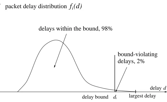
4.1 packet delay distribution and delay bound . . . 64

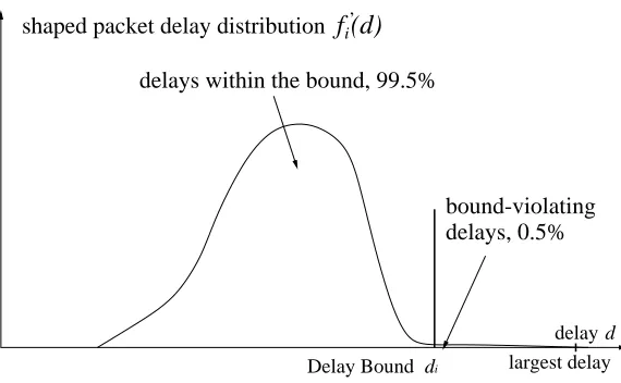
4.2 shaped packet delay distribution of flowi . . . 66

4.3 Inevitable deadline-violation period (t1, t2) . . . 68

4.4 QEDF Scheduling . . . 73

4.5 A general model for extending QEDF . . . 74

4.6 QEDF and EDF percentiles with ρ= 0.909 . . . 79

4.7 QEDF and EDF percentiles with ρ= 0.786 . . . 81

4.8 The second level of dynamics of AQE scheduling . . . 83

4.9 AQE Scheduling . . . 84

4.10 The AQE scheduling algorithm . . . 86

4.11 Mean Vector Field . . . 95

4.12 Mean Vector Field and Lyapunov Stability . . . 98

5.1 cell transmission table . . . 118

(13)

Chapter 1

Introduction

In this dissertation, we study packet scheduling algorithms in high speed networks that are targeted at statistical delay bounds. This chapter describes the general problem under study. Section 1.1 introduces modern computer networks and the next generation of integrated-service networks. Section 1.2 motivates the need of Quality of Service (QoS) in integrated-service networks and identifies packet scheduling algorithms as one of the most important mechanisms to deliver a very important QoS metric: packet delay bounds. Section 1.3 discusses some fundamental aspects of delay bounds and packet scheduling. Section 1.4 presents an overview of the dissertation.

1.1 Communication Networks

1.1.1 Packet Switching Networks

(14)

which deploy circuit switching, computer networks use packet switching as the underlying technology for information transportation.

In circuit switching, a physical communication channel (circuit) will be reserved and dedicated to end users throughout the life time of the communication; once the channel is established, the communication QoS will be guaranteed. However, the channel bandwidth may not be fully utilized if the communication is not active all the time, for example, when the people on a telephone conversation stop talking. For most applications of computer networks, the information data are not generated at constant rates, i.e., the applications are not at constant levels of activity all the time. Thus circuit switching has been considered as an inefficient technology for computer networks, given the fact that historically channel bandwidth has been limited and very expensive.

In packet switching, digitized information is split into small pieces called packets. Packets of many different communication sessions can be statistically multiplexed onto a physical channel in order to better utilize the bandwidth. In addition to this statistical mul-tiplexing gain on bandwidth, packets can be easily processed by computers, thus numerous services can be provided on the top of a packet-switched network.

1.1.2 Integrated-Service Networks

Traditionally, packet networks only provided data services like email, telnet and

(15)

real-time/interactive in nature. Consequently the traffic content in today’s packet networks, notably the Internet, does not consist of pure data any longer, but more of those found in telephony networks and cable TV networks. This convergence of traffic content not only satisfies the physiological needs of human being, but also provides the great potential to develop new, complex and highly intelligent services, even those not envisioned today. Therefore, from applications’ standpoint, it is highly desirable to integrate voice, video and data services into a single network. On the other hand, with the tremendous progress in optical communications, bandwidth availability has been exponentially growing in the last several years and the growth is expected to continue in the near future, which ensures that it is technically feasible to integrate into the network many bandwidth-demanding applications like video conference and video-on-demand, even with a large customer base.

Although bandwidth is rapidly increasing, the bandwidth demand from applica-tions also increases correspondingly. It is very difficult to predict that in the future the total available bandwidth can satisfy all communication needs, including the most demand-ing case. With this vista and the fact that most envisioned future applications will still have variable, in many cases highly variable, data rates, packet switching probably will remain the technology-of-choice for information transportation, if not the ubiquitous one, for the emerging high speed integrated-service networks.

(16)

network, which is a huge nonlinear system with numerous feedback effects, the global traffic pattern becomes very complicated and unpredictable. Providing predictable QoS to those applications, then, becomes extremely difficult. We will elaborate on this QoS issue in the next section.

1.2 Quality of Service in Integrated-Service Networks

1.2.1 QoS Requirements from Applications

(17)

Real-time applications can be further classified into one-way communications (e.g., video-on-demand) or interactive communications (e.g., video telephony). For the former, the variation in packet delays, or thedelay jitter, is more important than the delay itself; while for the latter both the delay and the delay jitter are important. Notice that if the end-to-end packet delays have an upper bound, delay jitter will have a natural upper bound, but this jitter bound may be too loose if the delays do not have a lower bound and the upper bound is loose.

Packet losses are mainly caused by buffer overflow at switching nodes. There are two basic approaches to cope with this problem. The first is to retransmit a packet after the packet is lost; the second is to use buffer dimensioning and priority assignment at switching nodes to ensure that the packets of some applications will never be lost.

Since the packet loss problem can always be solved by packet retransmissions, the QoS requirements from best-effort applications (i.e., packet loss and throughput) can be accommodated within a relatively large time frame. In contrast, the very nature of real-time applications dictates that their primary QoS requirements (delay and delay jitter) must be satisfied within a much smaller time frame. Therefore, in integrated-service networks it is more difficult to provide QoS to real-time applications than to best-effort applications, and the former are usually considered to have higher priority than the latter. The central topic of this dissertation is about packet scheduling algorithms which can directly control packet delays, thus we discuss packet delays in greater details below.

(18)

transmission delay and queueing delay at each switching node, and the signal propagation delay along the route of the packet. Among these delay components, only the queueing delay has great variation and is difficult to control or predict, other delays can be mod-eled as constants. Therefore, without loss of generality, in this dissertation all the delay components other than the queueing delay are assumed to bezero.

When packets of many traffic flows arrive at an outgoing link of a switching node, possibly from many incoming links, because of the finite transmission capacity of the link and the randomness of packet arrivals, packets may not depart immediately and have to wait in a queue, hence queueing delays result. As a packet needs to travel through several switching nodes before reaching its destination node, the end-to-end queueing delay of the packet is the summation of the local queueing delays. From packets to packets, the variation in the end-to-end delays result in delay jitters. From now on we will call queueing delays simply as delays. Providing end-to-end delay bounds to real-time applications is one of the most important QoS requirements for future high speed networks.

1.2.2 The Effect of Traffics on QoS

(19)

is extremely difficult and there is no easy way (e.g., real measurement) to verify such model-ing. What is worse is that switching nodes are highly nonlinear queueing systems and they may distort traffic characteristics even further, making the modeling of traffic processes inside the networks intractable.

1.2.3 QoS Support from Networks

Given the very different QoS requirements from applications and the high uncer-tainty of traffic behaviors of those applications, it becomes very difficult for an integrated-service network to provide QoS. The network architecture should contain at least the fol-lowing five components (see [78], we rephrase the component functionalities here):

1. Flow Specification represents a contract (for a specific meaning of this in the context of ATM networks, see [3]) between a source node and the network which specifies both source traffic characteristics and negotiated QoS requirements.

2. Resource Reservation reserves network resources such as link bandwidth and buffer space in order to guarantee the QoS contract.

3. Call Admission Control (CAC) decides if the resource reservation and/or QoS contract should be accepted or rejected, based on some criteria.

(20)

5. Packet Scheduling decides the transmission order of packets in a waiting queue at an outgoing link of a switching node.

Although the precise set of QoS-supporting functions that the network should provide is arguable, the five components above identify the major methodologies towards QoS solutions that have been widely agreed upon in the research community. There exists some dependence among these components. The functions routing and CAC heavily depend on the particular choices of packet scheduling algorithms and resource reservation methods within the network, while the latter two components are tightly coupled. Also, packet scheduling, resource reservation and flow specification are mutually dependent. We explain this dependence below.

Routing and CAC algorithms are typically at the network layer, while packet scheduling algorithms are at the link layer (for the concept of layering in computer networks, see the excellent textbook [9]). When both routing and CAC algorithms are QoS-aware at the packet level, that is, when routing becomes QoS routing [4] and CAC is targeted at packet-level QoS (packet delays and packet losses, in contrast to call-level QoS such as the call blocking probabilities in telephony networks), the performance of lower layer algo-rithms (packet scheduling and buffer management) must be known before routing or CAC algorithms can be executed. In this sense, routing and CAC depend on packet scheduling algorithms.

(21)

These two kinds of algorithms are related [38], as for a given flow, more bandwidth allo-cated to it, less buffer space required by it; equivalently, larger packet delays tend to result in more packet losses, which is in line with the famous Little’s law of classical queueing theory [41].

Packet scheduling and resource reservation are tightly coupled. To see this, we notice that the very purpose of scheduling algorithms is to provide delay QoS to traffic flows via bandwidth management. In order to make such a QoS provisioninga priori, some form of bandwidth reservation, either explicit or implicit, is indispensable, as otherwise the random background traffic flows may destroy the QoS during the bandwidth competition process. On the other hand, how bandwidth should be reserved critically depends on the performance of the scheduling algorithms chosen. Another condition needed to make such a delay QoS provisioning a priori is some form of source traffic regulation, as without it (in which case source nodes could generate traffic arbitrarily) the bandwidth reservation becomes meaningless. Therefore, it takes packet scheduling, resource reservation and source traffic regulation all together to provide delay QoS. This coupling in turn determines how the flow specification (QoS contract) should be made. The relationship among these functions and delay QoS provisioning can be understood in Fig. 1.1. The queueing system in Fig. 1.1 can be considered as either local (a switching node) or end-to-end (a tandem of switching nodes).

(22)

resource reservation bandwidth

link scheduling

system queueing

enforced BW resource guarantee

+

delay QoS delivered output flows with regulated traffic

input flows with

Figure 1.1: Delay QoS provisioning

delay bounds to real-time applications.

1.3 Providing Delay Bounds by Packet Scheduling

Basically, scheduling is the process of assigning transmission priorities (order of transmission) to packets, and different schedulers differ in their ways of priority assign-ments. Obviously, the order of transmission will significantly affect the delays experienced by individual packets.

1.3.1 Delay Bounds: Deterministic and Statistical

(23)

deterministic bounds the schedulable regions [30] are inherently conservative and small [60]. On the other hand, as discussed in Section 1.2.1, many real-time applications typically can tolerate a small percentile of packet losses, thus they can tolerate a small percentile of long packet delays as a packet loss trivially equals to an infinite packet delay. Therefore, a practical and very desirable solution for delay QoS is to provide statistical delay bounds.

For a statistical delay bound, there are possibly many definitions for it, and it is not easy to justify a particular choice of definition. For example, the definition could be either in a “at steady state” sense or in an “over specific intervals” sense [46], where the former has an ideal theoretical meaning and the latter has a very practical meaning. As an example of the issue, suppose 1% of a flow’s packets violate some given end-to-end delay bound, then whether those violations are in a row or in bursts or uniformly distributed throughout the life time of the flow makes a significant difference to the communication quality perceived by the end users; therefore a simple statement like “1% of the packets violate the delay bound” is somewhat vague. Here the real difficulty in choosing a definition is that we are trying to fit a complex real system (a network, all of whose numerous parameters, including the life time of flows, are finite) into a pure probabilistic model,and the performance evaluation of this model must generate practical meaning to the real system.

(24)

d∗ is within the bound, i.e., d∗ ≤ di, and the packet is late if d∗ > di. Let Ai(t) be the

accumulative amount of traffic from flowiin bytes by timet, among which Gi(t) bytes are

good, then we say the time-dependent quantity

pi(t) =

Gi(t)

Ai(t)

(1.1)

is the percentile function of good packets of flowiat time t. If

lim inf

t→∞ pi(t)≥pi, (1.2)

then we say flow i has a delay bound di with percentile pi, or percentile bound {di, pi}.

Notice that pi(t) is actually a function of the delay bounddi, thus we use notationpi(t, d)

to emphasize this dependence on a particular choice of delay bound d and use pi(t) to

specifically meanpi(t, di). We make two observations here. First, in the definition we do not

assume the convergence ofpi(t). If all percentile functions{pi(t)}indeed converge, then we

will have a stable system and this is very desirable. However, even if the percentile function

pi(t) converges, we do not know whether pi(t, d) converges for an arbitrary delay bound

d, so this single percentile convergence is even weaker than weak convergence (convergence in distribution, see [12]). Second, how the packet delays within the bound di are actually

(25)

1.3.2 Workconserving v.s. Non-workconserving Schedulers

In general, packet schedulers can be classified as workconserving schedulers or non-workconserving schedulers. For a good survey on schedulers by this classification, see [76]. A workconserving scheduler will schedule packets whenever there are some packets waiting in the queue. In contrast, a non-workconserving scheduler could become idle even when there are some packets waiting. In the context of integrated-service networks these definitions are implicitly assumed to be with respect to real-time packets; a non-workconserving scheduler could avoid wasting bandwidth by scheduling best-effort packets when it “becomes idle”, but from the viewpoint of real-time packets, the scheduler is still non-workconserving.

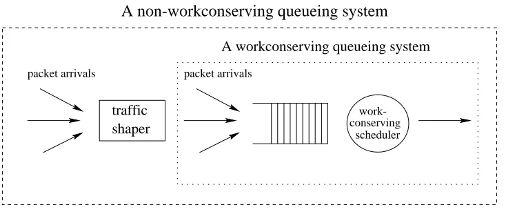
The primary objective of using non-workconserving schedulers is to control the traffic burstiness seen at local switching nodes. Once the burstiness is under control thus more predictable, it will be easier to provide local, thus end-to-end, delay bounds. Typically, a non-workconserving scheduler is implemented with a workconserving scheduler and a traffic shaper (see Fig. 1.2). The shaper will enforce some artificial packet delays so that when packets leave the shaper to the scheduler, their burstiness conforms to some traffic regulation specifications.

1.3.3 Scheduling: Rate Reservation v.s. Delay Budget Distribution

(26)

packet arrivals packet arrivals

traffic shaper

work-conserving scheduler

A workconserving queueing system

A non-workconserving queueing system

Figure 1.2: Implementation of a non-workconserving scheduler

limit the traffic generation rate as well as the traffic burstiness magnitude at the source node (cf. Fig. 1.1). In this case, it is better to consider the route of the flowas a whole, or a direct pipe, instead of isolated switching nodes; the task of packet scheduling becomes to guarantee the reserved rate ateach node. If the end-to-end bound is considered as a delay budget, then delay bound guarantee becomes to efficiently spend this budget and prevent it from being depleted. A naive solution towards this is to distribute the end-to-end budget into local budgets (delay bounds) at each switching node along the route of the flow, then guarantee those local delay bounds by packet scheduling. In this case, switching nodes are considered as isolated from each other.

(27)

Rate (GR) schedulers [35] which, as the name tells, can guarantee a flow a rate. EDF, on the other hand, has a known schedulability (delay bound guarantees, see [48]) condition for LB-regulated traffic flows at asingle node, and is known to be optimal with respect to this schedulability. It has been shown that with per-node traffic shaping EDF schedulers can provide end-to-end delay bounds and outperform WFQ in the sense of schedulable region [29]. The overall policy of this shaping/EDF scheme is named as Rate-controlled EDF (RC-EDF).

Although WFQ (GR) and RC-EDF scheduling can provide deterministic delay bounds, both schedulers have to consider the worst-case traffic scenario in order to guar-antee rates or local delay bounds. As discussed in the last subsection, the approach of deterministic delay bounds is very conservative in terms of bandwidth utilization, and to many real-time applications statistical delay bounds are more suitable. To our best knowl-edge, no practical packet scheduler has been proposed in the literature to provide statistical delay bounds; the current solution in the research community is to investigate some well-known schedulers like WFQ and RC-EDF for statistical delay bounds [22] [60]. However, we argue that such an effort is both ad hoc and ineffective because those schedulers are not designed in the first place to cope with traffic burstiness, the very source that drives the deterministic bounds loose.

(28)

guarantee local delay bounds. The solution of WFQ has the flavor of circuit switching, which indeed guarantees QoS by dedicated communication channels (thus transmission rates); while the solution of RC-EDF keeps the philosophy of packet switching, i.e., per-node packet processing. Because delay bounds (instead of transmission rates) are the ultimate delay QoS goal for real-time applications, the delay budget distribution approach (RC-EDF) is direct while the rate reservation approach (WFQ) isindirect. An understanding of this point will help to effectively design scheduling algorithms that can provide statistical delay bounds. We will elaborate on these two principles of resource reservation in Chapter 2.

1.4 Overview of the Dissertation

In this research, we study packet scheduling algorithms that are targeted at sta-tistical end-to-end delay bounds. We will show that our proposed new schedulers are better suited to provide statistical delay bounds than well-known schedulers like WFQ and RC-EDF. We emphasize here that in general providing statistical end-to-end delay bounds is a very tough and still open problem, any complete solution towards it must include not just packet scheduling algorithms, but also traffic regulation and CAC algorithms, which are difficult problems in their own rights. Therefore in this study we do not intend to provide an overall solution.

(29)

In Chapter 3, we present Deadline-curve based EDF (DC-EDF) scheduling, which does not use traffic shapers but can still provide deterministic end-to-end delay bounds and a schedulable region at least as large as that of RC-EDF. DC-EDF not only works in a natural work-conserving way, but also is self-adaptive in local delay bound assignments. When providing statistical bounds is the delay QoS objective, DC-EDF is very suited for scheduling at the intermediate nodes along a flow’s route. We also prove in this chapter that another EDF-based scheduling policy known in the literature, which does not use traffic shapers either, can also provide deterministic end-to-end delay bounds and a schedulable region as large as that of RC-EDF.

In Chapter 4, we propose Adaptive Quasi-EDF (AQE), which is an enhancement of EDF with intelligence of adaptive scheduling. AQE behaves like EDF when bandwidth is sufficient (i.e., no deadline-violation happens), but in the case of bandwidth deficiency, it only schedules a subset of flows which currently have relatively worse performance; other flows are completely blocked and will be unblocked only when bandwidth becomes sufficient again. Essentially, AQE enforces shaping on packet delay distributions and reduces the aggregate number of deadline-violations. AQE is most suited for scheduling at “the last hop”, i.e., at a switching node when all flows competing for bandwidth are at their last switching nodes. AQE combined with DC-EDF can provide an end-to-end solution for statistical delay QoS.

(30)

distribute any excess bandwidth within short periods in a controllable way, thus have the great potential to control delay jitters. GDGRQ can be used when both statistical delay bounds and minimum bandwidth guarantees are needed, which could be a very practical requirement.

(31)

Chapter 2

End-to-end Delay Bounds: A

Strategic Analysis

(32)

ideas instead of complicating our discussion by unnecessary technical complexity, we assume in this Chapter that traffic flows are fluid, i.e., they have infinitely small packet sizes.

2.1 Graphical Understanding of End-to-end Delays

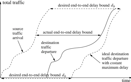
Although the actual queueing delays within a network are complicated, the delays seen by a pair of end users and their relationship with a requested end-to-end bound are conceptually simple, which can be understood from Fig. 2.1.

db

destination source

ideal destination with costant traffic

arrival

departure traffic

actual end-to-end delay bound

maximum delay

time total traffic

desired end-to-end delay bound

traffic departure

Figure 2.1: End-to-end delay and the ideal parallelogram

(33)

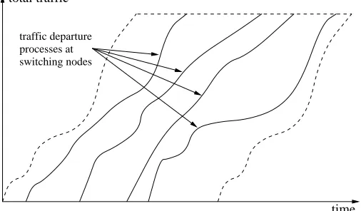
destination, the queueing/scheduling process will generate local departure processes of dif-ferent “shapes”, as shown in Fig. 2.2. It is clear that the control over the end-to-end delays will beessentially broken into controls over these local departure processes.

time total traffic

traffic departure processes at switching nodes

Figure 2.2: End-to-end delay and local departure processes

Notice that the departure process at a switching node will be the arrival process at the next switching node, which results in the traffic dependence within the network. For a local departure process, denoted byS(t), it has two distinct properties that are controllable. One is the “timing” of the process and the other is the “shape” of the process. With timing-control, the exact occurrence time ofS(t) will be bounded. For example, ifDl(t) andDu(t)

are some given lower bound and upper bound on the timing ofS(t), respectively, thenS(t) needs to satisfy

Du(t)≤S(t)≤Dl(t). (2.1)

(34)

“unpre-dictably”. A well-known and well-accepted method for such shape-control is Leaky Bucket, a special case of the so-called subadditive envelope control [13].

LetAi(s, t) be the total amount of traffic from flow iarriving over interval [s, t],

s ≥ 0, and define Ai(t) = Ai(0, t). Let A∗i(t), A∗i(t) = 0 for t ≤ 0, be a nondecreasing

subadditive process [13]. If

Ai(s, t)≤A∗i(t−s) (2.2)

for any interval [s, t], then A∗_i(t) is said to be an envelope of flowAi(t) andAi(t) is said to

conform toA∗_i(t), denoted byAi(t)A∗i(t). IfA∗i(t) =ρt+σ, whereρ and σ are positive,

then Ai(t) is said to be regulated by a LB; if A∗i(t) = min{ρ1t+σ1, ρ2t+σ2}, typically

with ρ1 > ρ2 >0 and σ2 > σ1 = 0, then Ai(t) is said to be regulated by a double LB. A

subadditive envelope process consisting of multiple linear segments, like the double LB, is relatively easy to be enforced.

Notice that if the timing of a departure process is controlled by both an upper bound and a lower bound, then there exists a degenerate shape-control on the process, as the process can not behave with arbitrary burstiness. Thus it is possible to make both timing-control and shape-control at a switching node, which we will see when we discuss RC-EDF scheduling in Chapter 3. If the timing is only controlled by an upper bound, which essentially serves as a deadline process for the departure process (i.e., Du(t)≤S(t)), then

(35)

2.2 Scheduling: from Local Control Perspective

The timing-control and shape-control over local departure processes discussed in the last section are consistent with the principles of network resource reservation discussed in Section 1.3.3. In particular, the timing-control is related to delay budget distribution and the shape-control is related to rate reservation. We explain these in the rest of this section.

2.2.1 Scheduling with Delay Budget Distribution

If the timing of a local departure process is under control (see Eq. (2.1)), then the packet delays from the source node to the local node are also under control and fairly predictable (cf. Fig. 2.2). Usually, at a switching node only an upper bound on the local departure process is needed, because early packet departures will not be harmful. At the destination node, however, a lower bound on the timing may also be desired because of delay jitter concerns. The approach of timing-control, when used for end-to-end delay control, essentially breaks an end-to-end delay bound into a sequence of local departure deadline processes, and the very task of packet scheduling is to guarantee those local deadlines. This is exactly the approach of delay budget distribution.

(36)

Under the EDF scheduling, each flowi is assigned a local delay bound di at the

scheduler; a packet j of flow iarriving at time ai,j is assigned a deadline

Di,j =ai,j+di. (2.3)

Packets are sent in the increasing order of their deadlines with arbitrary tie-breaking rules. However, the deadlines can not be guaranteed if packets arrive at arbitrary times. If arriving traffics have been regulated, in particular, if Ai(t) A∗i(t) for each i and some envelope

A∗_i(t), then the necessary and sufficient condition [48] for {Ai(t), di} to be schedulable is

known to be

X

i

A∗_i(t−di) +lmaxI_{dmin≤t<dmax} ≤ct, fort≥0, (2.4)

wherecis the link capacity, lmax is the maximum packet size of all flows, dmin = mini{di},

dmax = maxi{di}and I_{E} is the indicator function of event E.

The key feature of a GR scheduler is that it can guarantee transmission rates to in-dividual flows. This GR property is defined through a concept called GR Clock (GRC) [35]. Suppose a flow i reserves a rate ri on a link of normalized capacity 1 at a scheduler. Let

ai,j and di,j be the arrival and departure time of the jth cell of the flow i. The GR Clock

(GRC) of the cell is defined as: GRCi,0 = 0, GRCi,j = max{ai,j, GRCi,j−1}+ 1/ri. The

scheduler belongs to the GR class if

(37)

for each flow i and packet j, where βi, called the latency of flow i, is a constant and

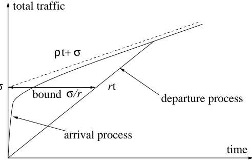
independent of any pattern of flow arrival processes. The GRC values represent some conditional deadlines of packet departures, where the conditioning is on (1) packet arrival times, (2) the history of packet arrivals and (3) the rate guaranteed by the scheduler. This is in sharp contrast with the case under EDF, where the deadline assignments depend only on the packet arrival times and are otherwise independent of the scheduler (see Eq. (2.3)). If flow i has been regulated by a LB with envelope A∗_i(t) = ρ(t) +σ, then a local delay boundσ/ri can be guaranteed to the flow by a GR scheduler withβi= 0, provided ri ≥ρ.

This can be understood from Fig. 2.3.

σ

t+ σ

ρ

bound _{departure process}

time total traffic

arrival process

r

σ/r t

Figure 2.3: The delay bound under a GR scheduler

Although a GR scheduler can provide local delay bounds, those bounds are con-ditioned on the rates guaranteed by the scheduler. If at each switching node a local bound

(38)

schedulers [76]; in contrast EDF scheduling does not have this delay/bandwidth coupling problem. Second, the switching nodes are considered as isolated from each other, the traffic dependence among the nodes has not been exploited. To get around this second problem and utilize the traffic dependence, the route of a flow should be considered as a direct pipe, instead of isolated nodes. As we discussed in Section 1.3.3, this approach is in line with the rate reservation principle, which we will discuss in the next subsection. We make the conclusion that although GR schedulers can provide local delay bounds, they are not proper for the delay budget distribution approach towards end-to-end delay control.

2.2.2 Scheduling with Rate Reservation

We have discussed that rate reservation is a principle towards end-to-end delay control. This is not as conceptually evident as the delay budget distribution approach. A natural question is what is the relationship between the rate reservation principle and the end-to-end delays that we understood from Fig. 2.2. In Fig. 2.3 we have already perceived a sense about the local delay bounds provided by a GR scheduler, now we investigate the end-to-end case in Fig. 2.4.

(39)

db db time

total traffic

r > ρ,at any switching node envelope

local departure processes 1 2 3

R(t)=rt

A guaranteed rate r, A Leaky Bucket

desired end-to-end delay bound

ρt+σ

σ

Figure 2.4: Local departure processes with a guaranteed rater

flow encounters a congested node and barely receives the reserved rater at that node, then the local departure process will experience large packet delays, which is the case of process-2 in Fig. process-2.4. However, process-process-2 becomes “smooth” after node-process-2 and will not experience large delays at the next switching node, even the flow again barely receives the reserved rate at the next node. This is the case of process-3 in Fig. 2.4.

Therefore, with rate reservation the traffic dependence between adjacent switching nodes is explicitly exploited; once packet experience large delays at a bottleneck node, the delays at subsequent nodes will be small; the end-to-end delays will have an upper bound, which is determined by the “shape” of the source arrival process and the reserved rate. In Fig. 2.4, in order to meet the desired end-to-end bounddb, R(t) must be no later than

(40)

the envelope ρt+σ, a careful observation of Fig. 2.4 will conclude that this requirement will be satisfied if and only if

r ≥max{ρ, σ db

}, (2.6)

and the actual end-to-end delay bound ¯dwill be simply

¯

d=σ/r. (2.7)

All the GR schedulers mentioned in the last subsection provide deterministic bounds ac-cording to the two equations above. If the source traffic is regulated by a double LB or a general subadditive envelope, Eq. (2.7) will be slightly modified, but fundamentally remain the same.

(41)

2.3 Statistical Delay Bounds Oriented Scheduling

Providing deterministic end-to-end delay bounds has been well understood in the literature, manifested by the extensive results on GR-class schedulers [51] [52] [74] [34] [35] [71] [25] [62] and EDF-based schedulers [29] [30] [48] [26] [49]. As discussed in Section 1.3.1, deterministic delay bounds are very conservative in terms of bandwidth utilization and statistical delay bounds are more desirable. In general providing statistical delay bounds is a difficult problem due to the uncertainty on the statistical characteristics of source traffic arrivals and the complicated traffic behavior within the network. Heuristically, if a tight statistical (percentile) delay bound is desired for a flow, then for the packet delays of the flow that are within the bound, i.e., for the delays of good packets (see the definitions in Section 1.3.1), they should

1. be as close to the bound as possible, and

2. have jitters as small as possible.

The justification for these heuristics is that, as we pointed out in Section 1.3.1, how the packet delays within the bound are actually distributed isnot important to the percentile delay bound {di, pi} (see Eq. (1.2)). Therefore, larger those good-packet delays are, less

(42)

be loose if there is no lower delay bound and the upper bound is loose. Here we observe the reverse implication, i.e., small jitters imply a smallrange of delay values, which leads to tight statistical bounds.

For the first heuristic, i.e., to make good-packet delays as close to the bound as possible, the delays are clearly meant to be end-to-end. Therefore, the scheduling control following this heuristic should primarily exist at the last switching node along a flow’s route. A scheduler well-designed for this end should be able to actively control the delays of individual packets. We will see how this can be done when we study AQE scheduling in Chapter 4.

For the second heuristic, i.e., to make packet delay jitters as small as possible, the traffic dependence among adjacent switching nodes should be exploited. The intuition behind this argument is simple: as the end-to-end delay jitters are trivially the summation of local delay jitters, large local delays at a switching nodes can be balanced with small local delays at other switching nodes to prevent the end-to-end delay jitters from building up. This is true for both deterministic and statistical delay bounds, as we have already observed in Section 2.2.2 how a GR scheduler utilizes this idea in a straightforward way to make its deterministic delay bounds tight. We argue in this dissertation that this idea can be implemented in more sophisticated ways, for both the delay budget distribution approach and the rate reservation approach that we discussed in Section 2.2.

(43)

actual delays the packets of that flow have experienced before arriving at the local node. The scheduler can then make its scheduling decisions based on the information to control the delay jitters seen at the local node. We will see how this can be done when we study DC-EDF scheduling in Chapter 3.

(44)

Finally in this chapter, we remark that, as we pointed out in Section 1.3.3, the de-lay budget distribution approach is more direct than the rate reservation approach towards end-to-end delay control. Under the latter approach, it is not easy to obtain analytical results on the delays of individual packets (e.g., local packet delay distributions) directly from the reserved rates. As a consequence of this, we have not been able to find a proper mathematical framework to quantitatively analyze the packet delay correlations among ad-jacent switching nodes where rate-reservation-based schedulers are deployed, especially if the schedulers have the intelligence of adaptive scheduling, as the case of GDGRQ sched-ulers.

(45)

Chapter 3

Deadline-curve Based Earliest

Deadline First Scheduling

3.1 Introduction

(46)

delay bounds is problematic because inside a network traffics will be distorted and local schedulability conditions will be violated. Although rate-controlled EDF was proposed as early as in [24] and [40], it was not known then if this idea can be exploited for EDF to provide end-to-end delay bounds. Meanwhile, WFQ with its many variations became very popular as they provide strong traffic isolations thus can deliver end-to-end delay bounds regardless of the internal traffic burstiness of a network.

The idea of per-node traffic shaping was first formalized in [29] with a solid the-oretical foundation. The authors of [29] showed that with identical shapers at each node along a flow’s path, EDF not only provides tight deterministic end-to-end delay bounds, but also outperforms WFQ; the new policy was named RC-EDF. Although shaper delays will not worsen the end-to-end delay bounds [29] and RC-EDF can still work in an en-forced work-conserving way (see Section VI in [29]), traffic shaping does introduce artificial packet delays. When statistical delay bounds are needed, artificial delays may make the statistical bounds worse, or equivalently, make the schedulable region smaller. There are two major reasons for the need of statistical delay bounds for RC-EDF. First, network-wide EDF schedulability conditions are very difficult to guarantee (for a sense of this, see [26]). Second and more importantly, as we discussed in Chapter 1, since the schedulability condi-tions consider the worst traffic scenario ateach node, the delay dependency along a flow’s path is not sufficiently exploited and the resulting schedulable region is inherently very con-servative [60]. Another drawback of RC-EDF is that shaper implementations are typically complicated [60].

(47)

shaper delays, are really indispensable in order to provide the end-to-end delay bounds. In this chapter, we propose a deadline-curve based EDF scheduler (DC-EDF) which does not use shapers, but assigns packet deadlines differently from that assigned by RC-EDF. Specifically, under DC-EDF local deadlines are chosen as time-shifted versions of source packet arrival times. We show that DC-EDF can also guarantee deterministic end-to-end delay bounds and can provide a schedulable region at least as large as that of RC-EDF. Under DC-EDF, if a packet misses its deadline at some node due to a local schedulability condition failure, its queueing priority at the next node will be automatically enhanced since the next deadline is independent of its arrival time. DC-EDF scheduling not only follows the delay budget distribution principle we discussed in Chapter 1 and Chapter 2, but also follows the heuristic to reduce the delay jitters seen at local switching nodes that we discussed in Chapter 2. These properties make DC-EDF attractive to provide statistical delay bounds. By using techniques developed in the chapter, we will also address an unsolved problem in the literature. Specifically, we prove that an EDF-based scheduling policy previously proposed in the literature which does not use traffic shapers can also guarantee deterministic end-to-end delay bounds and provide a schedulable region at least as large as that of RC-EDF.

(48)

Section 3.7 we summarize the chapter.

3.2 Previous Works

3.2.1 Rate-Controlled EDF

As any schedulers, EDF may distort traffic characteristics in the scheduling/queueing process. To keep flows locally schedulable, a rate-control mechanism can be added to an EDF scheduler. Basically there are two ways to add the rate-control functionality, which we call RC Method-1 and Method-2. Method-1, which is used in RC-EDF, inserts a traffic shaper associated with an envelopeA∗_i(t) before the EDF scheduler for each flowi, then uses Eq. (2.3) to assign deadlines (cf. Fig. 1.2). Thus when flow icomes to the EDF scheduler, it has been enforced by the shaper to conform to A∗_i(t). If a flow already conforming to an envelopeI(t) goes through a shaperA∗(t), then there is a maximum shaper delay [29] and it is denoted by D(IkA∗). It was shown in [29] that D(IkI) = 0. Also, [29] showed the important result that if a flow i conforming to Ii(t) goes through identical shapers A∗i(t)

at each node k along its path and a local delay bound di,k is guaranteed at node k, then

the enforced delays in thekth shaper will not introduce any delaybeyond the delay bounds guaranteed at node k; instead, the shaper delays just compensate the queueing delays and the total delays are still within the bounds. It is shown in [29] that the end-to-end delay bound to the flow is

¯

di=D(IikA∗i) + Ki

X

k=1

(49)

whereKi is the number of nodes that flowitravels through.

It should be noticed that although Eq. (2.4) is the necessary and sufficient condition of local schedulability for an EDF scheduler, due to its complexity, a practical RC-EDF system will use the following sufficient condition for local schedulability tests (see Eq. (3) in [38] and Eq. (26) in [26]):

X

i

A∗_i(t−di) +lmax≤ct, fort≥dmin (3.2)

We comment here that RC-EDF scheduling not only controls the timing of lo-cal departure processes (by deadline guarantees), but also controls the shape of them (by explicit traffic shaping). This is possible because, as we discussed in Section 2.1, timing-control with both upper bound and lower bound will yield a degenerate shape-timing-control; the traffic shaping enforced by RC-EDF exactly realizes this lower bound on the timing of a local arrival process (regarded as a departure process from the previous node).

RC Method-2, proposed earlier [24] [40] than Method-1, neither explicitly deploys shapers nor directly uses Eq. (2.3) to assign local deadlines. Instead, it computes deadlines after taking into account the envelope of an arriving flow. In the simple case [24] [40] where only a peak rate is applied for traffic regulation (i.e., by a LB withρ >0 andσ = 0), packet deadlines are recursively assigned [76] as

Di,j = max{ai,j +di, Di,j−1+Ximin}, (3.3)

(50)

rate (i.e., Xmin

i = 1/ρ). The resulting scheduling policy is work-conserving. The idea of

Method-2 is that no delay will be enforced to packets even the packets are burstier than allowed by their envelopes; the burstiness will be accommodated by deadline assignments which equal to that of the same flow under RC Method-1, i.e., as if the flow will be shaped by its envelope first. Therefore, as discussed in [49], both RC Method-1 and Method-2 assign thesame deadlines to individual packets, but differ in how they handle the potential earliness [49] of a packet. Method-1 enforces additional delay to balance the earliness while the Method-2 simply allows earliness. To our knowledge, however, in the literature there is no result on if RC Method-2 can really guarantee end-to-end delay bounds. The necessary and sufficient condition in [48] can not be used directly because under RC Method-2 traffic arrival processes are not shaped and may not conform to their envelopes. In Section 3.5 we will prove that although without traffic shaping, RC Method-2 can indeed guarantee end-to-end delay bounds, and its schedulable region is at least as large as that of RC-EDF (Method-1).

3.2.2 Service Curve Based EDF

(51)

RC Method-1 and Method-2 [58]. It has been shown that with flexible selection of SCs SCED has strictly larger schedulable region than RC-EDF [58]. However, it is unclear if this enlargement is significant and can justify the involved deadline computations. SCED is very deterministic-delay-bound-oriented and seems hardly allowing statistical delay bounds.

3.3 DC-EDF Scheduling

3.3.1 Motivations

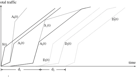
For a given flow, ideally all its packets should experience the same end-to-end delay. If some packets experience large delays but others experience small delays, then the earliness of the less-delayed packets is undesirable; it not only consumes bandwidth inefficiently (i.e., some “delay budget” is wasted) but also introduces delay jitters. As we discussed in Section 2.3, the most effective approach to cope with this jitter problem is to balance large local delays at some nodes with small local delays at some other nodes, by which hopefully the end-to-end delays will have less jitter and bandwidth is used more efficiently. Both RC methods discussed in the last section partially achieve this objective, but not in a “best-effort” way. Intuitively, the “best-effort” way should assign deadlines at their “latest allowable” times. This suggests that at an EDF scheduler deadlines should be chosen as a time-shifted version of the source packet arrival times, regardless of the actual traffic arrival times at the scheduler. We graphically illustrate this intuitive idea below.

In Fig. 3.1, flowi has accumulative source arrival process A0(t) and needs to go

(52)

1

2

time

1

d d

D (t)2

I(t) (t) (t) 1 A (t) 1 S (t) A (t) D 0 A 2 1 D’(t)2 total traffic

Figure 3.1: Different deadline assignments

the arrival process becomesA1(t); then the deadline process forA1(t) isD1(t) =A1(t−d1).

Due to the effect of queueing/scheduling, the departure process at the first scheduler is

S1(t). At the second scheduler, S1(t) is shaped to A2(t) and the corresponding deadline

process is D2(t) = A2(t−d2). Here we observe that the shape of A2(t) is quite different

from that of A1(t) and A2(t) is well ahead of D1(t). This reveals that even with shapers,

flows deep inside the network could still be very different from what they are at their first switching nodes, and they could arrive far ahead of their latest allowable arrival times. However, from the viewpoint of deterministic delay bound guarantees, any traffic earliness is useless, and the earliness should be definedwith respect to the guaranteed bounds.

In [49], under RC-EDF traffic earliness is defined as the time between a distorted flow and its shaped version, e.g., betweenS1(t) andA2(t) in Fig. 3.1; the delays in the shaper

only compensate for this earliness. Consequently, in Fig. 3.1 the deadline processD2(t) at

the second node is well ahead ofD₂0(t) =D1(t−d2) =A1(t−d1−d2), the actual delay bounds

(53)

toD0₂(t), other flows at the second scheduler would have better chance (more bandwidth) to meet their deadlines. This is important if the global schedulability condition fails and statistical delay bounds are being sought. Our proposed DC-EDF scheduling exploits this idea.

3.3.2 System Model, Definitions and Notations

We assume there is a set N = {1,2,· · · , N} of flows in the network, each is connection-oriented and has a known routing path of Ki nodes which does not contain a

loop. The accumulative amount of source traffic of flow i over interval [0, t] is denoted by

A(0)_i (t). Suppose under a RC-EDF system, each flowiwill go through a shaper of envelope

A∗_i(t) at thekthnode in its path and will be guaranteed a local delay bounddi,kat the EDF

scheduler, where 1≤k≤Ki. To be in line with the model used in [29] in order to compare

a DC-EDF system with a RC-EDF system, under DC-EDF scheduling we assumeA(0)_i (t) is instantaneously shaped toA(1)_i (t) at the source so that A_i(1)(t) A∗_i(t). Also, each packet

j of flow iis assigned a deadline

D_i,j(k)=a(1)_i,j +

k

X

n=1

di,n (3.4)

at its kth node, where a(1)_i,j is the arrival time of packet j at its first switching node, as determined byA(1)_i (t). Accordingly, we say the deadline curve of flow iat itskth node is

D(_ik)(t) =A(1)_i (t−

k

X

n=1

(54)

Formally, under a DC-EDF system each link of a switching node will use an EDF scheduler, with packet deadlines assigned as above. We assume that throughout the network, DC-EDF schedulers use arbitrary but fixed tie-breaking rules; the tie-breaking rules are considered as an integrated part of EDF scheduling.

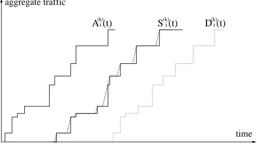
Let A(_ik)(t) and S_i(k)(t) denote the accumulative arrival and departure processes over [0, t], respectively, at the kth node of flowi. By convention switching is assumed to be non-cut-through, thus A(_ik)(t) is a right continuous step function where a jump will occur whenever the last bit of a packet arrives. Once a packet arrives completely, it may start transmission immediately. It is easy to see that larger A(_ik)(t) means earlier packet arrivals of flow iand vice versa. We will model A(_ik)(t), S_i(k)(t) and D(_ik)(t) precisely, i.e., not by fluid model; they are graphically shown in Fig. 3.2.

time aggregate traffic

(t) (k)

Ai S(k)i(t) D(k)i(t)

Figure 3.2: Arrival process, departure process and deadline curve

(55)

easy to see that for all i and k, if S_i(k)(t) ≥D(_ik)(t) for all t ≥0, then the deadline curve

D(_ik)(t) is satisfied.

Although for a link with capacity c the total available bandwidth over interval [0, t] is ct, we allow the link to beon vacation (e.g., serving best-effort packets) from time to time. The length of a vacation is limited to be the transmission time of integer many bytes. With link vacations we denote the available bandwidth over interval [u, v] byC(u, v) and define the bandwidth function (BF) of the link as C(t) = C(0, t). Notice that C(t) is a continuous function. In theory with an arbitrary BF, packets may not be transmitted continuously; but the scheduler by itself is still non-preemptive (i.e., packet-by-packet) and simultaneous transmission of multiple packets is not allowed. In practice all packets will be transmitted continuously because BFs areactually generated from real queueing systems.

3.4 Global Schedulability under DC-EDF

Despite that traffic burstiness is not directly controlled in a DC-EDF system, in this section we show that a DC-EDF system can provide end-to-end delay bounds and a schedulable region at least as large as that of RC-EDF. We first examine DC-EDF at a single node.

3.4.1 The Single Node Case

(56)

A careful examination on Eq. (3.2) reveals that the key of this schedulability condition is that packet deadlines, instead of arrivals, should not be “too bursty”; also it turns out that in Eq. (3.2) deadlines happen to be time-shifting of arrival times. This suggests that under DC-EDF, if deadline curves are not “too bursty” and packets arrive “early enough”, then the deadline curves should be schedulable.

Let Ai(u, v) be the amount of traffic from flow i arriving over the close interval

[u, v]. Notice that since Ai(t) is right continuous, Ai(u, v) = Ai(v)−Ai(u−). We define

urgent trafficEi(u, v) as the amount of traffic of flowithat arrive afteru−and has deadlines

no later thanv. Easily,

Ei(u, v) = max

0, Di(v)−Ai(u−) . (3.6)

The urgent trafficEi(u, v) represents the bandwidth demand from flow iwithin the interval

[u, v].

SupposeFis the set of flows arriving at a link with BFC(t) andlmaxis the largest

packet size of all flows, we have the following sufficient condition for local schedulability at a DC-EDF scheduler:

Theorem 3.1. A sufficient condition for deadline curves {Di(t), i∈ F} to be schedulable,

i.e.,Si(t)≥Di(t) holds for all i∈ F and all t≥0, is that for any interval [u, v], u≥0,

X

i∈F

Ei(u, v)≤max{0, C(u, v)−lmax}. (3.7)

(57)

deadline and packet size of the kth _{packet (of any flow) that departs from the queueing}

system by ak, sk, fk, dk and lk, respectively. Let the first deadline-violation happen at

time fn, i.e., at the time of the nth departure, thus fn > dn. Let am be the last time

before fn when a busy period begins, obviously m exists and am =sm. Let e = max{k :

m ≤ k ≤ n;dk > dn}. If e does not exist, then dk ≤ dn, for all k, m ≤ k ≤ n, but

Pn

k=mlk ≤

P

i∈FEi(am, dn) ≤max{0, C(am, dn)−lmax} ≤C(am, dn), so it is impossible

that fn > dn, a contradiction, thus e exists; let the corresponding packet be e. Then,

each packet of thekth departure,e+ 1≤k≤n, has deadlines smaller thane but departs later than it, thus they all arrive after time se. Thus 0<

Pn

i=e+1li ≤

P

i∈FEi(se, dn) ≤

max{0, C(se, dn)−lmax} and we have

Pn

i=eli ≤max{le, C(se, dn)−lmax+le} ≤C(se, dn),

hence it is impossible thatfn> dn, a contradiction again. Therefore,fndoes not exist and

no deadline violation will ever happen.

Remark 3.1. In this theorem there is no burstiness constraint on any individual deadline curveDi(t). By Eq. (3.6), if the packets of a flowiarrive earlier (i.e. Ai(t)larger),Ei(u, v)

will be smaller and Eq. (3.7) will be easier to hold.

Remark 3.2. Although Eq. (3.7) is a sufficient condition for the schedulability of{Di(t), i∈

F}, examples can be easily given to show that it is not a necessary condition. However, it

is close to the necessary condition given below.

Theorem 3.2. A necessary condition for deadline curves {Di(t), i∈ F} to be schedulable

is, for any interval [u, v], u≥0,

X

i∈F

(58)

Proof: Suppose for some interval [u, v],u >0,P_i_∈FEi(u, v)> C(u, v). By

defini-tion,P_i_∈FEi(u, v) is the total amount of packets that arrive afteru−and have deadlines no

later thanv, but the total available bandwidth over [u, v], C(u, v), is less than this amount of traffic, therefore some deadline-violations are inevitable over [u, v]. Eq. (3.7) differs from Eq. (3.8) only by the termlmax, which is introduced by the

non-preemptive nature of EDF scheduling. In this sense, the sufficient condition in Theo-rem 3.1 is analmost-necessary condition for the local schedulability at a DC-EDF scheduler. The following example of traffic pattern illustrates that the condition in Theorem 3.2 isnot sufficient for local schedulability under DC-EDF.

Example: Suppose the condition in Theorem 3.2 holds and for some interval [u, v], 0 < C(u, v)−lmax < P_i_∈FEi(u, v) ≤ C(u, v). Also suppose for some flow j, Ej(u, v) =

0. Let a packet e from flow j with size l = lmax and deadline D > v arrive and start

transmission at time u − (the link is idle before u −), where c < P_i_∈FEi(u, v)−

(C(u, v)−lmax). By definition

P

i∈FEi(u, v) is the total amount of traffic from F that

arrives afteru− and has to depart no later than v, but since the total bandwidth available over [u, v] is justC(u, v) and the transmission ofecan not be preempted, it can be checked that a deadline-violation will occur.

The following corollary decouples the simultaneous constraints onAi(t) andDi(t)

(59)

Corollary 3.1. If for each i∈ F, Ai(t)≥Di(t+di) and for any interval [u, v], u≥0,

X

i∈F

max n

0, Di(v)−Di (u+di)−

o

≤ max0, C(u, v)−lmax , (3.9)

then the deadline curves {Di(t), i∈ F} are schedulable.

Proof: For any i ∈ F and any interval [u, v], since Ai(t) ≥ Di(t +di), we

have max{0, Di(v) −Ai(u−)} ≤ max{0, Di(v) −Di((u+ di)−)}, thus

P

i∈FEi(u, v) ≤

P

i∈Fmax{0, Di(v)−Di((u+di)−)} ≤max{0, C(u, v)−lmax}, by Theorem 3.1, the deadline

curves{Di(t), i∈ F} are schedulable.

The next corollary can be immediately concluded from Corollary 3.1.

Corollary 3.2. If the deadline curves {Di(t), i∈ F} satisfy the condition in Eq. (3.9) for

all i∈ F but a deadline-violation occurs at time tv, the departure time of a packet v, then

there is some packetj of some flowi, which arrives at timeai,j andDi,j−di < ai,j ≤tv−∆t,

where Di,j is the deadline of i, as determined by the deadline curve Di(t), and ∆t is the

transmission time of a single byte on the link.

Proof: Let packet v start transmission at time ts, then ts ≤ tv −∆t. Now we

modify the queueing system by supposing for any i ∈ F, Ai(t) = Ai(ts) for t ≥ ts, i.e.,

all traffic inputs are cut off at time t+_s. Obviously the corresponding modified deadline curves will still satisfy the condition in Eq. (3.9). Since all traffic flows remain unchanged before t+_s, with this modification all queueing activities remain unchanged before time t+_s

(60)

for which Ai(t) ≥ Di(t+di) does not hold over [0, ts], thus for some packet j of flow i,

Di,j−di< ai,j ≤ts≤tv−∆t. Corollary 3.2 says that if the condition in Eq. (3.9) holds, then any deadline-violation must be caused by some late arrival(s) strictly before the deadline-deadline-violation. This fact will be very useful when we show the global schedulability of a DC-EDF system.

3.4.2 Global Schedulability of DC-EDF

Now for notations we restore their dependencies on nodes and we index all links in the network by 1,2, ...J. Let the capacity of link j be cj and let Fj denote the set of

flows going through this link. For i∈ Fj, let link j be at thekthi,j node in the path of flow

i. We have the following theorem.

Theorem 3.3. Under a DC-EDF system, if for any linkj,P_i_∈F

jA

∗

i(t−di,ki,j)+lmax≤cjt

fort≥mini{di,ki,j}, then the deadline curves{D

(k)

i (t)},1≤i≤N,1≤k≤Ki, are globally

schedulable.

It can be seen that this global schedulability condition is the same as that of RC-EDF (see Eq. (3.2)). To prove Theorem 3.3, it suffices to show the following stronger lemma:

Lemma 3.1. If for any link j with BF Cj(t) and for any interval [u, v], u≥0,

X

i∈Fj

max n

0, D(ki,j)

i (v)−D

(ki,j)

i (u+di,ki,j)−

o

(61)

then{D_i(k)(t)}, 1≤i≤N, 1≤k≤Ki, are globally schedulable.

Proof of Theorem 3.3: Recall that A(1)_i (t) A∗_i(t) and D_i(k)(t) = A(1)_i (t−

Pk

n=1di,n). For any link j and interval [u, v], we have

D(ki,j)

i (v)−D

(ki,j)

i (u+di,ki,j)

−

= A(1)_i (v−

ki,j

X

n=1

di,n)−A(1)_i (u+di,ki,j −

ki,j

X

n=1

di,n)−

≤ A∗_i(v−u−di,ki,j) (3.11)

for each i∈ F. Thus

X

i∈Fj

max n

0, D(ki,j)

i (v)−D

(ki,j)

i (u+di,ki,j)

−o

≤ X

i∈Fj

max0, A∗_i(v−u−di,ki,j)

= X

i∈Fj

A∗_i(v−u−di,ki,j)≤cj(v−u)−lmax

≤ max{0, cj(v−u)−lmax}, (3.12)

then by Lemma 3.1 the theorem holds.

It can be seen that the condition Eq. (3.10) in Lemma 3.1 is essentially the same as the local schedulability condition Eq. (3.9) in Corollary 3.1, so intuitively Lemma 3.1 should easily hold if A(_ik)(t) ≥ D_i(k)(t+di,k) holds network-wide. However, this last condition is

(62)

exists a global schedule of packet arrivals/departures (possibly with deadline-violations). Suppose the very first network-wide deadline-violation occurs at time tv, the departure

time of packet v at link k. Consider the queueing activities on link k over the interval [0, tv]. Since the link capacity and local deadline curves satisfy Eq. (3.10) thus Eq. (3.9),

by Corollary 3.2 there exists a packet j of flow isuch that Di,j−di < ai,j < tv, where ai,j

and Di,j are the arrival time and local deadline of packetj at link k, respectively, anddi is

the local delay bound of flowiat linkk. Since at the first switching node of flowiwe have

a(1)_i,j =D(1)_i,j −di,1, link k can not be at the first switching node of flow i, so packet j must

come from some previous link k0 along the path of flowi. However, by Eq. (3.5) Di,j−di is

just the local deadline of packetj at linkk0. Sinceai,j is also the departure time of packet

j at link k0, this means packet j violates its local deadline at link k0 at time ai,j < tv, a

contradiction to the assumption that the first global deadline-violation occurs at time tv.

Therefore no deadline-violation will ever happen throughout the network.

3.5 Delay Bounds under a RC Method-2 System

(63)

end-to-end delay bounds. We first formally define a RC Method-2 system (cf. [49]).

Definition 3.1. In a RC Method-2 system, at each link an EDF scheduler is used and no shaper is used. For an arriving flow, its packet deadlines are assigned the same as if the packets arrive at a RC-EDF switching node, i.e., as if the packets are shaped by a corresponding envelope first and then assigned deadlines by a constant delay bound.

In the definition above, the shaper envelope of a fictitious RC-EDF scheduler is used to assign packet deadlines for the RC Method-2 system. However, it should be noticed that such a deadline equivalence only has meaning locally, i.e., at that switching node with a fictitious RC-EDF scheduler; in general the resulting packet deadlines within a RC Method-2 system are different from the deadlines that may result in if thewhole network is a RC-EDF system. The rest of our system model and notations are consistent with those in the previous sections. Under the RC Method-2 system, at link j let the accumulative arrival and departure processes of flow i, i∈ Fj, be A

0₍_k i,j)

i (t) and S

0₍_k i,j)

i (t), respectively,

where link j is at the kth_i,j node in the path of flow i. Let the deadline curve of flow i at link j be D0(ki,j)

i (t), then the arrival process A

0₍_k_i,j₎

i (t) will be first fictitiously shaped to

D0(ki,j)

i (t+di,ki,j) and then assigned the deadline curveD 0₍_k_i,j₎

i (t). We have

A_i0(ki,j)(t)≥D_i0(ki,j)(t+di,ki,j), (3.13)

D0(ki,j)

Statistical Delay Bounds Oriented Packet Scheduling Algorithms in High Speed Networks

Algorithms in High Speed Networks

by

Kai Zhu

A dissertation submitted in partial satisfaction

of the requirements for the degree of

Doctor of Philosophy

in

Computer Engineering

in the

Graduate School

of

North Carolina State University

Raleigh, 2000

Biography

Acknowledgements

Contents

List of Tables

List of Figures

Chapter 1

Introduction

1.1

Communication Networks

1.1.1

Packet Switching Networks

1.1.2

Integrated-Service Networks

1.2

Quality of Service in Integrated-Service Networks

1.2.1

QoS Requirements from Applications

1.2.2

The Effect of Traffics on QoS

1.2.3

QoS Support from Networks

+

1.3

Providing Delay Bounds by Packet Scheduling

1.3.1

Delay Bounds: Deterministic and Statistical

1.3.2

Workconserving v.s. Non-workconserving Schedulers

1.3.3

Scheduling: Rate Reservation v.s. Delay Budget Distribution

1.4

Overview of the Dissertation

Chapter 2

End-to-end Delay Bounds: A

Strategic Analysis

2.1

Graphical Understanding of End-to-end Delays

2.2

Scheduling: from Local Control Perspective

2.2.1

Scheduling with Delay Budget Distribution

2.2.2

Scheduling with Rate Reservation

2.3

Statistical Delay Bounds Oriented Scheduling

Chapter 3

Deadline-curve Based Earliest

Deadline First Scheduling

3.1

Introduction

3.2

Previous Works

3.2.1

Rate-Controlled EDF

3.2.2

Service Curve Based EDF

3.3

DC-EDF Scheduling

3.3.1

Motivations

3.3.2

System Model, Definitions and Notations

3.4

Global Schedulability under DC-EDF

3.4.1

The Single Node Case