Simple Molecule Mercury Sensor

ABSTRACT

WAN, YANJUN. Simple Molecule Mercury Sensor. (Under the direction of Dr. Christopher B. Gorman.)

Several molecules previously produced from a nitrile-based cascade cyclization were

examined as potential mercury sensors. Various analytical parameters, including fluorescence

quantum yield, UV shift, fluorescence quenching, binding constant, binding ratio, and lowest

detection limit, were measured. The best mercury sensor molecule was found to be molecule

3c, which could be easily synthesized in gram quantities (3 steps, 55% overall yield). This molecule has a very high fluorescence quantum yield (Φ = 0.87), high sensitivity and

selectivity towards mercury ion in both organic and aqueous media. The overall performance

Simple Molecule Mercury Sensor

by

Yanjun Wan

A thesis submitted to the Graduate Faculty of

North Carolina State University

In partial fulfillment of the

Requirements for the degree of

Master of Science

Chemistry

Raleigh, North Carolina

2008

APPROVED BY:

______________________________

Christopher Gorman

Committee Chair

______________________________

Stefan Franzen

______________________________

Edmond Bowden

DEDICATION

Seek first his kingdom and his righteousness, and all these things will be given to you as

well.

BIOGRAPHY

Yanjun Wan was born in China in the year of 1983. She attended elementary school,

middle school, and high school in China, and graduated high school with straight As. After

high school, Yanjun attended Shanghai Jiao Tong University. In June 2005, Yanjun

graduated from Shanghai Jiao Tong University with a Bachelor of Science degree in

Chemistry, and a Bachelor of Arts degree in Finance as double-major. To further her

knowledge in Chemistry, Yanjun decided to go to graduate school at North Carolina State

University, where she pursued a Master of Science degree in Chemistry under the direction

ACKNOWLEDGMENTS

I would like to first thank my parents for their love and support, despite of the distance

between us. I would also like to thank Berk and Barbara Wilson, who are like my parents in

Raleigh, for bringing light to my life, and teaching me the righteous way of living through

life’s up-and-downs, and for their constant love, care, and encouragement.

I would like to thank Dr. Christopher B. Gorman for being the most wonderful advisor I

could ever imagine. He taught me not just Chemistry, but a whole series of life philosophy,

which is eventually even more important than Chemistry; when I look back, working for him

is one of my wisest decisions in life. I would also like to thank all members in my Advisory

Committee, Dr. Edmond Bowden, Dr. Stefan Franzen, and Dr. David Shultz, for always

being available and patient whenever I have any questions. I would like to thank the Gorman

Group. Every single one of them has always been helpful and encouraging to me. It was my

pleasure to be able to work with them. I would also like to thank Dr. Paul Boyle for X-ray

Structure Analysis, Dr. Matthew Lynton for Mass Spectroscopy Analysis, Dr. Lin He for

suggestions on fluorescence measurements. The Mercury Sensor Project was supported by

US Department of Energy (Grant DE-FG02-05ER46238). The Molecular Transistor Project

was supported by National Science Foundation (DMR-0303746).

I would like to thank my “brothers and sisters” in Raleigh, Sasha Movchan, Susan Pope,

and Alina Efremenko, for always being there when I cry or when I laugh, and for loving me

and always supporting me in front of others, yet never hesitating to point out my faults

TABLE OF CONTENTS

LIST OF TABLES ... vi

LIST OF FIGURES ... vii

LIST OF SCHEMES ... ix

INTRODUCTION ... 1

1.1 The Importance of Mercury Sensing ... 2

1.2 Four Major Categories of Mercury Sensors ... 2

1.3 Organic Dye Based Mercury Sensors –Advantages and Challenges ... 7

A SMALL MOLECULE MERCURY SENSOR ... 9

2.1 Introduction... 10

2.2 Results and Discussion ... 11

2.3 Conclusions ... 24

2.4 Experimental Section ... 27

MOLECULAR TRANSISTOR PROJECT ... 33

3.1 Introduction... 34

3.2 Results and Discussion ... 37

3.21 Synthesis and Characterization of Linker Molecules ... 37

3.22 Synthesis of Metal and Metal Oxide Nanoparticles ... 39

3.23 Ligand Exchange Experiments ... 39

3.3 Conclusion ... 43

3.4 Prospects for Synthesis of Nanoparticle Hetero-dimers and Hetero-trimers ... 43

3.5 Experimental Section ... 51

LIST OF TABLES

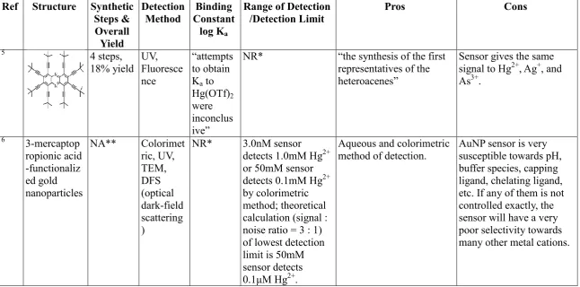
Table 1. A summary of recently reported mercury sensors. ... 3

Table 2. Photophysical data for 3b, 3c, 5b, and 5c. ... 14

Table 3. Different base systems for invariant concentration Job plot. ... 17

Table 4. Binding constant Ka of molecule 3c to different metal cations, calculated by

Benesi-Hildebrand plot. ... 21

Table 5. A quantitative comparison of molecule 3c to other promising organic dye based mercury sensors. ... 25

LIST OF FIGURES

Figure 1. X-ray crystal structures of 3b, 3c, 5b, and 5c. ... 12

Figure 2. Photograph of solutionsof0.1mM 3b, 3c, 5b, and 5c under UV light. ... 13

Figure 3. Electronic absorption spectra of 3b, 3c, 5b, and 5c in acetonitrile. ... 14

Figure 4. Fluorescence quantum yield calculation for 3b, 5b, 3c, and 5c in acetonitrile. ... 14

Figure 5. 0.5 mM molecule 3c mixed with 0.5 mM different metal cations, in 1% 0.2 M phosphate buffer and 99% acetonitrile. a) under day light; b) under UV lamp. ... 15

Figure 6. Invariant concentration Job plot of molecule 3c to mercury in acetonitrile. ... 16

Figure 7. Invariant concentration Job plot of molecule 3c to mercury in 1% aqueous buffer and 99% acetonitrile. ... 18

Figure 8. Suggested structure of the complex formed between molecule 3c and mercury nitrate. ... 18

Figure 9. A similar mercury complex characterized by X-ray diffraction by Ancker, et al.20 19 Figure 10. Binding of molecule 3c to mercury shows an obvious red shift upon increasing mercury concentration, in 0.5% 0.1 M phosphate buffer and 99.5% acetonitrile. ... 20

Figure 11. Addition of molecule 3c to mercury solution, where the concentration of mercury solution stays at 1 mM, while the concentration of molecule 3c solution varies from 0 to 50 µM. Solvent: 2% 0.25 M phosphate buffer and 98% acetonitrile. ... 20

Figure 12. Benesi-Hildebrand plot reveals the binding constant between molecule 3c and mercury: Ka = 4.94  104 M-1. ... 21

Figure 13. Structure comparison between molecule 3c and isoquinoline-3-amine. ... 22

Figure 14. Binding constant comparison between molecule 3c and isoquinoline-3-amine in 0.5% 0.1M phosphate buffer and 99.5% acetonitrile. Addition of molecule 3c incurred an obvious peak at 400 nm, but the same concentration of isoquinoline-3-amine did not incur any peak at 400 nm. ... 22

Figure 15. Oxygen dependent fluorescence quenching of molecule 3c. Flushing oxygen for 15 seconds reduced more than half of the fluorescence of molecule 3c, this quenching is reversible and the fluorescence of molecule 3c can be recovered upon flushing nitrogen. ... 23

Figure 16. Available thiophene molecules for future examination. ... 26

Figure 17. Proposed structures of water-soluble versions of molecule 3c. ... 27

Figure 18. A cartoon of the definition of (from left to right) homo-dimer, hetero-dimer, homo-trimer, and hetero-trimer. ... 35

Figure 19. a) TEM image of 7 nm iron oxide nanoparticles; b) Histogram of the size distribution of nanoparticles in a). ... 39

Figure 20. TEM images of iron oxide nanoparticle samples after ligand exchange with tartaric acid, showing (left) aggregated particles and (right) debris thought to result from aggregates of excess ligand that were not removed upon purification. ... 41

Figure 21. a) TEM image of 3nm gold nanoparticles capped by hexanethiol; b) Histogram of the size distribution of nanoparticles in a); c) TEM image of 3nm platinum nanoparticles capped by hexanethiol; d) Histogram of the size distribution of nanoparticles in c). ... 42

Figure 23. (a) The minimum linker length calculation for gold homo-trimer; (b) Structure and length of available three-arm homo-linker. ... 46

Figure 24. (a) The minimum linker length calculation for gold-iron oxide hetero-trimer; (b) Structure and lengths of the proposed three-arm hetero-linker. ... 47

LIST OF SCHEMES

Scheme 1. Synthesis of oligomer precursors. ... 11

Scheme 2. Cascade closure of multiple aromatic rings. ... 12

Chapter 1

1.1

The Importance of Mercury Sensing

There is an increasing concern over the severe risk of heavy metal pollution and

poisoning in environment, food, and products.1 Mercury ion is of particular interest because of its high toxicity and its ability to cause a wide variety of damage to the kidneys, digestive

system, and neurological system.2 Different forms of mercury can also be transformed between one another, under different environmental conditions.3 The most harmful form – methylated mercury, can become biomagnified up the food chain, reaching 106 – 107 times greater in some fish species, compared to the amount in surrounding water.4 Such high mercury levels can affect the health of animals at all stages in the food chain, including

humans.3 Thus, a simple yet highly-selective routine to detect mercury ions in both organic and aqueous media is of great interest.

1.2

Four Major Categories of Mercury Sensors

Most recently developed mercury sensors fall into one of four general categories:

nano-particle based sensors, DNA or other bio-molecule based sensors, polymer based

sensors, or organic dye based sensors. Table 1 summarizes several of these and indicates

Table 1. A summary of recently reported mercury sensors.

Ref Structure Synthetic Steps & Overall Yield Detection Method Binding Constant

log Ka

Range of Detection /Detection Limit

Pros Cons

5 _{4 steps,}

18% yield UV, Fluoresce nce “attempts to obtain Ka to

Hg(OTf)2

were inconclus ive”

NR* “the synthesis of the first representatives of the heteroacenes”

Sensor gives the same signal to Hg2+, Ag+, and As3+.

6 _3-mercaptop

ropionic acid -functionaliz ed gold nanoparticles

NA** Colorimet ric, UV, TEM, DFS (optical dark-field scattering )

NR* 3.0nM sensor detects 1.0mM Hg2+ or 50mM sensor detects 0.1mM Hg2+ by colorimetric method; theoretical calculation (signal : noise ratio = 3 : 1) of lowest detection limit is 50mM sensor detects 0.1μM Hg2+.

Aqueous and colorimetric method of detection.

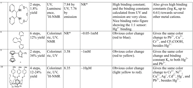
Table 1 continued…

7 _{2 steps,}

1.8% yield UV, Luminesc ence, 1_H-NMR 7.84 by UV, 7.76 by emission

NR* High binding constant; and the binding constants calculated from UV and emission are very close. Nice binding ratio figure showing the 1:1 sensor: Hg2+ binding.

Also gives high binding constants (log Ka up to

4.61) towards several other metal cations.

8 _{6 steps,}

12% yield

Colorimet ric, UV, NMR

NR* ~0.05-1mM Obvious color change (red to blue).

Gives the same color change to Pb2+, Cu2+, Cr3+, and CF3COOH,

besides Hg2+.

9 _{2 steps,}

34% yield

Colorimet ric, UV

3.58 ~1mM Obvious color change

(red to yellow).

Gives the same color change and binding constant Ka to both Hg2+

and Pb2+.

10 _{4 steps,}

12-24% yield

Colorimet ric, UV,

1_H-NMR

8.35 ~10μM Obvious color change

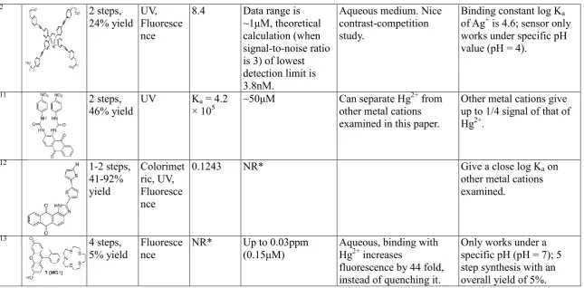
Table 1 continued…

2 _{2 steps,}

24% yield UV, Fluoresce nce

8.4 Data range is ~1μM, theoretical calculation (when signal-to-noise ratio is 3) of lowest detection limit is 3.8nM.

Aqueous medium. Nice contrast-competition study.

Binding constant log Ka

of Ag+ is 4.6; sensor only works under specific pH value (pH = 4).

11 _{2 steps,}

46% yield

UV Ka = 4.2

× 105

~50μM Can separate Hg2+ from other metal cations examined in this paper.

Other metal cations give up to 1/4 signal of that of Hg2+.

12 _{1-2 steps,}

41-92% yield Colorimet ric, UV, Fluoresce nce

0.1243 NR* Give a close log Ka on

other metal cations examined.

13 _{4 steps,}

5% yield

Fluoresce nce

NR* Up to 0.03ppm (0.15μM)

Aqueous, binding with Hg2+ increases

fluorescence by 44 fold, instead of quenching it.

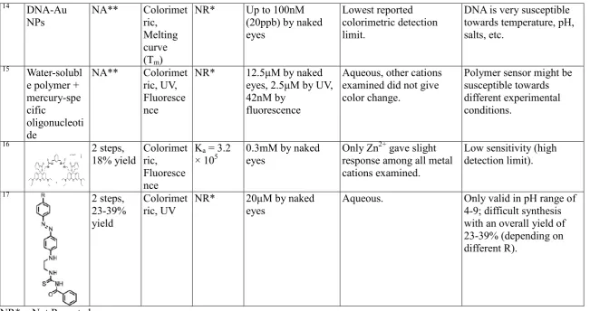
Table 1 continued…

14 _DNA-Au

NPs

NA** Colorimet ric, Melting curve (Tm)

NR* Up to 100nM (20ppb) by naked eyes

Lowest reported colorimetric detection limit.

DNA is very susceptible towards temperature, pH, salts, etc.

15 _Water-solubl

e polymer + mercury-spe cific

oligonucleoti de

NA** Colorimet ric, UV, Fluoresce nce

NR* 12.5μM by naked eyes, 2.5μM by UV, 42nM by

fluorescence

Aqueous, other cations examined did not give color change.

Polymer sensor might be susceptible towards different experimental conditions.

16 _{2 steps,}

18% yield Colorimetric, Fluoresce nce

Ka = 3.2

× 105 0.3mM by naked eyes Only Zn

2+ _{gave slight}

response among all metal cations examined.

Low sensitivity (high detection limit).

17 _{2 steps,}

23-39% yield

Colorimet ric, UV

NR* 20μM by naked eyes

Aqueous. Only valid in pH range of 4-9; difficult synthesis with an overall yield of 23-39% (depending on different R).

NR* = Not Reported.

While sensors in the first three categories usually have the advantage of lower detection

limit, their applications are highly constrained by their susceptibility to a series of factors，

including temperature, pH, and other salts. For example, DNA-functionalized gold

nanoparticles described by Lee, et al., showed the lowest reported colorimetric detection

limit of 100 nM (20 ppb) in aqueous media.14 However, two important components of this sensor, DNA and gold nanoparticles, are both known to show a large variability in their

behavior as a function of temperature, pH, and the presence of other salts. In fact, the whole

detection process required a thermal controller to control temperature between 46 ºC to 50 ºC.

Another example is the mercury sensor reported by Liu, et al., which used a water-soluble

conjugated polymer and a label-free, mercury-specific oligonucleotide probe.15 This sensor can detect different concentration ranges of mercury by different means – it has an aqueous

detection limit of 12.5 µM by colorimetric detection, 2.5 µM by UV, and 42 nM by

fluorescence. However, due to the sensitive and fragile nature of the polymer and the probe,

this sensor can hardly serve as an inexpensive way of detecting different forms of mercury in

a variety of environments.

1.3

Organic Dye Based Mercury Sensors –Advantages and Challenges

Unlike sensors in the first three categories, organic dye based sensors are usually

synthesized organic molecules with high fluorescence and remarkable optical changes upon

binding to mercury ions, with the potential advantages of low cost, easy storage, and better

based mercury sensors usually suffer from one or several disadvantages, including multi-step

synthesis with low overall yield; poor sensitivity and/or selectivity; low binding constant;

and poor aqueous solubility.

Some of the most convincing and potentially useful organic dye based mercury sensors

are: Mercury Green 1 synthesized by Yoon, et al., with a quantum yield of 0.72, and a

detection limit up to 0.03 ppm (0.15 μM) in aqueous medium;13 and azo-component containing chemodosimeters synthesized by Lee, et al., with a colorimetric detection limit of

4 ppm (20 μM) by naked eyes in aqueous medium.17 Unfortunately, both sensors require considerable amount of effort in synthesis, and are limited to use only in specific pH ranges.

Other various organic dye based sensors cited in Table 1 all have different drawbacks as well.

Some sensor molecules require long synthetic routes, and the overall yields are less than

20%.5,7,9,16 Some sensor molecules are poor at differentiating mercury from other metal ions, most commonly, zinc, cadmium, lead, copper, silver, etc.5,7-10 On top of these drawbacks, most organic dye based sensors can only detect mercury ions in organic solution.5,7-12 For the few molecules that are claimed to be able to respond to aqueous mercury, experiments were

performed in mixed solvent systems (usually acetonitrile : water or dimethylsulfoxide :

water).2,17

Thus, although many mercury sensing molecules and assemblies have been reported,

none is universally applicable or ideal. This lack has prompted the study of other molecules

Chapter 2

2.1

Introduction

For an organic dye based mercury sensor to be applicable in industry, the common

challenges listed in Chapter 1 have to be addressed properly. First of all, an easy synthetic

route for large scale synthesis with a decent overall yield is a must for industrial application.

Second, high selectivity of the sensor, especially the ability to differentiate mercury from

other commonly present metal cations, is also crucial. Third, a sensor that could detect

mercury ions in both organic and aqueous media would be highly preferred. Besides these,

high binding constant and low detection limit are also key parameters of the overall

performance. A large detection range and variety in detection methods (e.g. colorimetric, UV,

fluorescence, etc) are also helpful.

Our group recently discovered a new methodology to close multiple aromatic rings in

nitrile-containing oligomers in a cascade cyclization. This methodology involves the

synthesis of a series of nitrile-containing precursor oligomers, the acid-catalyzed cyclization

that are widely reported in the synthesis of isoquinolines,18 followed by the spontaneous tautomerization of CH groups to NH groups. To our knowledge, this new methodology is the

first to report cascade closure of multiple aromatic rings. A series of products synthesized by

this methodology exhibit high quantum yield, which can potentially be used as organic dye

based sensors for different heavy metal ions.

Presented below are several potential organic dye based mercury sensors (3b, 3c, 5b, and 5c) synthesized by this cascade cyclization methodology, and their performance as colorimetric sensors. Their electronic absorption spectra and quantum yield were examined

revealed the high selectivity of molecule 3c towards mercury ion, and a series of quantitative measurements, including UV shift, fluorescence quenching, binding ratio, binding constant,

and lowest detection limit in both organic and aqueous media, were performed to examine

the overall performance of molecule 3c as a potential mercury sensor.

2.2

Results and Discussion

As shown in Scheme 1, oligomers 3a and 5a can be easily synthesized from commercially available starting materials. These oligomers could then be converted to

cyclized products (Scheme 2) in which the benzylic CH groups were found to tautomerize to

NH. This process results in entirely aromatic rings. To our knowledge, this is the first

example of cyclization/aromatization of this kind. Full details of every synthetic step are

provided in the experimental section.

Scheme 1. Synthesis of oligomer precursors. CN CN

CN CN CN NC

Cl CN

+

ii NC

Cl CN

+

CN

1 2 3a (97%)

1 4 5a (73%)

i

Scheme 2. Cascade closure of multiple aromatic rings. CN CN

CN CN CN 3a

5a

N NH2

Br

N N NH₂ Br

i ii

N NH2

N N NH2

3b (72%) 3c (79%)

5b (59%) 5c (76%)

i ii

i) HBr/HOAc; ii) NaBH4, Pd on Carbon

Crystals of 3b, 3c, 5b, and 5c, suitable for X-ray diffraction, were obtained by group member Weijun Niu (Figure 1). These data showed that we were able to close multiple

aromatic rings in one step reaction, followed by debromination to reduce considerable steric

hindrance.

(3b) (3c) (5b) (5c)

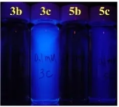
In Figure 2, solutions of 3b, 3c, 5b, and 5c at the same concentration (0.1 mM, in acetonitrile) showed considerable differences in fluorescence under UV lamp - the

debrominated 3c and 5c showed obviously higher fluorescence. For a sensor to operate via fluorescence quenching, a large quantum yield of fluorescence in the unbound form, and a

small quantum yield in the mercury bound form is desirable.

Figure 2. Photograph of solutionsof0.1mM 3b, 3c, 5b, and 5c under UV light.

The electronic absorption spectra of these 4 molecules are shown in Figure 3. One can

see that molecule 5c has a slightly higher extinction coefficient at virtually all wavelengths than other molecules. The quantum yields for fluorescence were determined in anhydrous

acetonitrile, between 375 nm and 600 nm. The results are shown in Figure 4 and Table 2.

Molecule 3c gave approximately 5 times higher quantum yield than molecule 5c. Based on quantum yield, molecule 3c was chosen as the most promising sensor for heavy metal ions among these molecules. Detailed procedures for obtaining electronic absorption spectra and

Figure 3. Electronic absorption spectra of

3b, 3c, 5b, and 5c in acetonitrile.

Figure 4. Fluorescence quantum yield calculation for 3b, 5b, 3c, and 5c in acetonitrile.

Table 2. Photophysical data for 3b, 3c, 5b, and 5c.

Compound Abs. Max Fl. Max  (Quantum Yield)

3b 378nm 447nm 2%

3c 370nm 436nm 87%

5b 348nm 450nm 3%

5c 346nm 432nm 15%

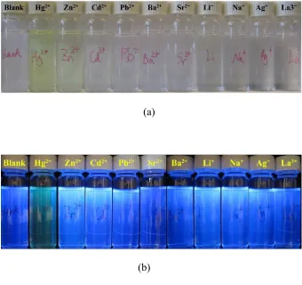
In qualitative tests, molecule 3c exhibited very high selectivity towards mercury ion. In Figure 5a, the vial with mercury nitrate showed an obvious color change from colorless to

dark yellow, while in Figure 5b, the vial with mercury nitrate showed almost completely

quenching of the fluorescence of molecule 3c. No other metal cations examined here exhibited the same color change or fluorescence quenching, qualitatively suggesting a high

(a)

(b)

Figure 5. 0.5 mM molecule 3c mixed with 0.5 mM different metal cations, in 1% 0.2 M phosphate buffer and 99% acetonitrile. a) under day light; b) under UV lamp.

To determine the stoichiometry of the molecule/mercury complex, an X-ray diffraction

showing the crystal structure of the molecule/mercury complex would be most desirable.

However, due to the low solubility and stability of the molecule/mercury complex in

common solvents, several attempts to obtain crystals suitable for X-ray diffraction were all

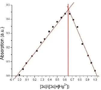
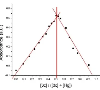
unsuccessful. Thus, an invariant concentration Job plot (Figure 6) was constructed. In this

plot, the absorbance of a series of acetonitrile solutions with the same total concentration, but

complete binding of all molecule 3c and all mercury ions available in solution. Solving

𝟑𝒄 ( 𝟑𝒄 + 𝐻𝑔2+ _{) = 0.65 gives the ratio of [3c]:[Hg}2+_{] = 2:1, indicating a 2:1}

stoichiometry of the molecule/mercury complex.

Figure 6. Invariant concentration Job plot of molecule 3c to mercury in acetonitrile.

This 2:1 stoichiometry was unexpected and not desirable. The stoichiometry is different

than most mercury/molecule complexes and thus, relative binding affinity cannot be

compared between this complex and others in the literature. Moreover, as two molecules are

required for each mercury ion, this stoichiometry consequentially requires more molecules to

get a response than is ideal. It was wondered what the role of the second equivalent of the

molecule was in the overall binding. Cotton et al. suggested a possible role. Specifically, it

was noted that “This ligand (Ammonia) reacts in a unique way with mercury(II)

compounds”19. As shown in equation 1.1,19 one of the ammonia acted merely as a proton acceptor. Thus, despite of a seemly 2:1 ratio of reacted ammonia to mercury, the binding

HgCl

+ 2NH

HgNH

Cl(s) + NH

+ Cl

This suggests to us that the 2:1 ratio initially observed in the invariant concentration Job

plot could be “misleading” in terms of revealing the true binding ratio between mercury and

molecule 3c. To test this possibility, an invariant concentration Job plot in the presence of excess base was proposed, in the hope that such excess base would be more favorable as the

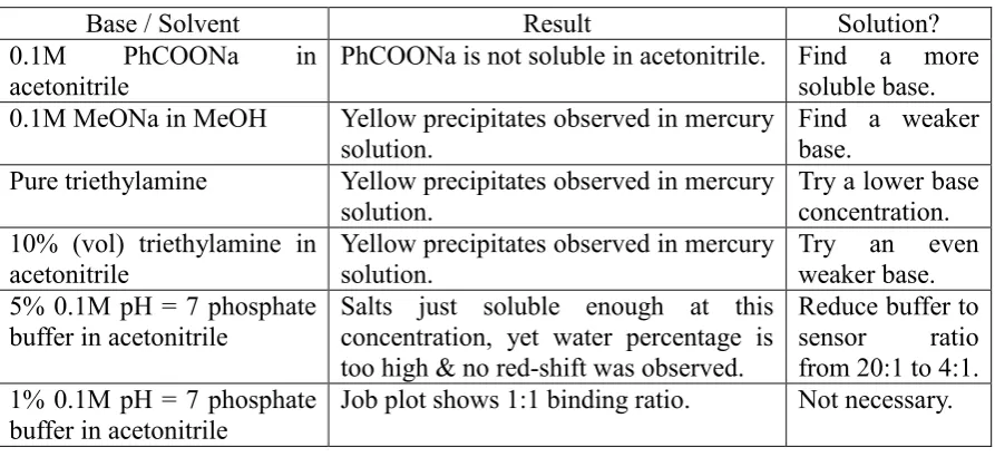
proton acceptors, thus molecule 3c would only be consumed as ligands to mercury complex. Table 3 shows the different base systems examined in sequence, and the reasoning for such

selections. As can be observed, selection of base and ionic strength were important in

obtaining a successful result.

Table 3. Different base systems for invariant concentration Job plot.

Base / Solvent Result Solution?

0.1M PhCOONa in

acetonitrile PhCOONa is not soluble in acetonitrile. Find a more soluble base. 0.1M MeONa in MeOH Yellow precipitates observed in mercury

solution. Find a weaker base.

Pure triethylamine Yellow precipitates observed in mercury solution.

Try a lower base concentration. 10% (vol) triethylamine in

acetonitrile

Yellow precipitates observed in mercury solution.

Try an even weaker base. 5% 0.1M pH = 7 phosphate

buffer in acetonitrile

Salts just soluble enough at this concentration, yet water percentage is too high & no red-shift was observed.

Reduce buffer to sensor ratio from 20:1 to 4:1. 1% 0.1M pH = 7 phosphate

buffer in acetonitrile

Finally, a Job plot in 1% aqueous buffer and 99% acetonitrile solution avoided the

consumption of molecule 3c as a sacrificial proton acceptor, and revealed a 1:1 binding ratio between molecule 3c and mercury complex, as shown in Figure 7. Under these conditions, a first order binding constant was then obtained. This result suggests a 4-member ring complex,

as shown in Figure 8. Such 4-member ring mercury complexes have been reported earlier by

Ancker, et al., and the structure of this mercury complex was characterized by X-ray

diffraction, as shown in Figure 9.20

Figure 7. Invariant concentration Job plot of molecule 3c to mercury in 1% aqueous buffer and 99% acetonitrile.

N NH

Hg NO3

Figure 9. A similar mercury complex characterized by X-ray diffraction by Ancker, et al.20

A qualitative test of binding revealed a ~40nm red-shift in the UV absorption peak when

molecule 3c was exposed to mercury ion (Figure 10). To calculate the binding constant Ka

from Benesi-Hildebrand plot, different concentrations of molecule 3c were added to mercury solutions of much greater concentration (Figure 11). Under these conditions, it is considered

that all molecule 3c added to the solution was bound to excess mercury, which has no absorption at 400 nm. Thus, the observed peak in corresponding UV spectra at 400 nm,

corresponds solely to the absorption of molecule/mercury complex. Figure 12 is the

Benesi-Hildebrand plot constructed from these data, and a Ka of 4.94  104 M-1 was

calculated. While zinc ion is the only cation that exhibited a small new peak around 410 nm,

corresponding to a Ka of 7.49  102 M-1, none of the other metal cations examined gave any

Figure 10. Binding of molecule 3c to mercury shows an obvious red shift upon increasing mercury concentration, in 0.5% 0.1 M phosphate buffer and 99.5% acetonitrile.

Figure 12. Benesi-Hildebrand plot reveals the binding constant between molecule 3c and mercury: Ka = 4.94  104 M-1.

Table 4. Binding constant Ka of molecule 3c to different metal cations, calculated by

Benesi-Hildebrand plot.

Metal Cation

Hg2+ Zn2+ Li+, Na+, K+, Ag+, Cd2+, Pb2+, Co2+, Ca2+, Sr2+, Ba2+, La3+, Tl3+

Ka( ) 4.94  104 7.49  102 Too small to measure by this method

However, the structure of molecule 3c resembles that of the commercially available

isoquinoline-3-amine. As shown in Figure 13, molecule 3c has one more substituent benzene ring, which provides extra electron density. Such an increase in electron density was later

proven to be crucial for the sensing of mercury ion: as shown in Figure 14,

isoquinoline-3-amine did not respond to the same concentration of mercury ion, but molecule

3c incurred an obvious peak at 400 nm, corresponding to a Ka of 7.49  102 M-1, as reported

N NH2 N NH2

molecule 3c isoquinoline-3-amine

Figure 13. Structure comparison between molecule 3c and isoquinoline-3-amine.

Figure 14. Binding constant comparison between molecule 3c and isoquinoline-3-amine in 0.5% 0.1M phosphate buffer and 99.5% acetonitrile. Addition of molecule 3c incurred an obvious peak at 400 nm, but the same concentration of isoquinoline-3-amine did not incur any peak at 400 nm.

The binding constant Ka ofmolecule 3c to mercury ion could also be measured by

Stern-Volmer plot. However, because oxygen is a much stronger fluorescence quencher than

(Figure 15) shows that flushing oxygen for 15 seconds reduced more than half of the

fluorescence from molecule 3c solution. Thus, the whole procedure of obtaining Stern-Volmer plot, which involves exposure of molecule 3c solution to air/oxygen for much longer than 15 seconds, would inevitably introduce a great error in the amount of quenched

fluorescence by oxygen, and thus produce a much greater error in calculated binding constant

Ka.

Figure 15. Oxygen dependent fluorescence quenching of molecule 3c. Flushing oxygen for 15 seconds reduced more than half of the fluorescence of molecule 3c, this quenching is reversible and the fluorescence of molecule 3c can be recovered upon flushing nitrogen.

The lowest detection limit of molecule 3c to mercury ion was found to be approximately 0.1 ppm (0.5 μM) in both organic (acetonitrile) and aqueous (dimethylsulfoxide:water = 4:1)

sensing studies, where molecule 3c and mercury ion were mixed with the same concentration of Li+, Na+, K+, Ag+, Cd2+, Pb2+, Co2+, Ca2+, Sr2+, Ba2+, La3+, and Tl3+, molecule 3c displayed the same lowest detection limit, which further illustrated its high selectivity towards mercury

ion.

2.3

Conclusions

To date, four different molecules have been successfully synthesized as possible

mercury sensors. The most promising mercury sensor among them was found to be molecule

3c, which can be easily synthesized in grams (3 steps, 55% overall yield), yet has a very high fluorescence quantum yield (Φ = 0.87), high sensitivity and selectivity towards mercury ion

in both organic and aqueous media. The binding constant of molecule 3c was found to be 4.94  104 M-1 to mercury, but only a maximum of 7.49  102 M-1 to all other metal cations examined.

Molecule 3c also showed considerable advantages over two of the most promising organic dye based sensors13,17 reported in recent literature, as shown by the comparison given in Table 5. Among these sensors, molecule 3c is much easier to synthesize with a much higher overall yield. Although binding constants of the other two molecules were not

reported, the binding constant of molecule 3c is comparable to or greater than any others reported. Molecule 3c is also highly selective towards mercury ion, demonstrated by the mixed ion sensing experiment above; and its selectivity towards mercury ion can be

suggest that molecule 3c is a very promising organic dye based mercury sensor.

Table 5. A quantitative comparison of molecule 3c to other promising organic dye based mercury sensors.

Sensor Molecule

CN CN

CN CN CN 3a

5a

N NH2

Br

N N NH2

Br

i ii

N NH2

N N NH2

3b (72%) 3c (79%)

5b (59%) 5c (76%)

i ii

Reference 13 17 This work (3c)

Synthesis _{overall yield} 4 steps, 5% 2 steps, 23-39% _{overall yield} 3 steps, 55% _{overall yield} Binding Constant Ka NR* NR* 4.94  104

Detection Method & Limit

Colorimetric NR* 4 ppm (20 μM) 20 ppm (100 μM)

Fluorescence 0.03 ppm (0.15 _μM)** NR* 0.1 ppm (0.5 μM)** NR* = Not reported

**: Both detection limits are measured at signal/noise = 3/1 ratio.

Some preliminary results suggest possible routes for the continuation of this project. A

series of molecules with fused aromatic rings were synthesized by this methodology, and

could be modified in different ways to make potential sensors for different metal cations. For

example, several thiophene molecules shown in Figure 16 were successfully synthesized and

characterized by group member Weijun Niu. Their photophysical and binding properties to

Figure 16. Available thiophene molecules for future examination.

Moreover, because the performance of molecule 3c as a mercury sensor did not decrease in the presence of water as a potential competing reagent, a water soluble version of

molecule 3c is proposed in

Figure 17. Such structures employed the hydrophilic -SO3Na group to increase the

solubility of the whole sensor in aqueous medium, yet retained the crucial structure to

mercury binding (the 2-aminopyridine function with high electron density). These proposed

molecules could be synthesized and examined as potential aqueous mercury sensors. The fact

that the mercury sensor itself is water soluble would allow a completely aqueous testing of

mercury waste in aqueous systems; and a lot of other solvents can be tested, as the extinction

Figure 17. Proposed structures of water-soluble versions of molecule 3c.

2.4

Experimental Section

General Considerations

All chemicals were purchased from Aldrich or Acros. Acetonitrile was dried by

distillation over CaH2. Anhydrous dichloroethane in a sure seal bottle was purchased from

Acros and used without further drying. Tetrabutylammonium hexafluorophosphate (TBAPF6)

was recrystallized three times from ethanol. Mercury nitrate monohydrate was used as

mercury source in all concerning measurements. All synthesis steps below were firstly

examined and characterized by group member Weijun, Niu. The buffer concentrations were

chosen at a minimum level (4:1 ratio) to both provide excess “proton acceptor” and minimize

a decrease in the solubility of molecule 3c in mixed solvent system.

Synthesis of 3a. To a flask containing 822.9 mg (7.4 mmol) of potassium tert-butoxide in 10 mL dimethylformamide (DMF), cooled in an ice bath, a mixture of 656.0 mg (4.8

mmol) 2-chlorobenzonitrile (1) and 430.4 mg (3. 7 mmol) 2-phenylacetonitrile (2) in 6 mL DMF was added drop wise. The reaction mixture was then stirred at room temperature (RT)

for 1 h, after which 20 mL saturated ammonium chloride (aq.) was added to quench excess

deionized water (DI), and dried over anhydrous sodium sulfate. Column purification with

dichloromethane (DCM) and gradient addition of methanol, followed by removal of solvent

and further drying under vacuum gave light yellow crystals (780.1 mg, 97% yield).

Alternatively, this reaction was carried out on a larger scale (6.6 g, 71% yield) and the

column purification step was replaced by recrystallization from hot ethanol.

Synthesis of 3b. To a flask containing 625.5 mg (2.9 mmol) of 3a, 7 mL of 45% HBr in acetic acid was added. The resulting solution turned yellow and was stirred at RT for an

additional 2 h. A 10 mL portion of ethyl acetate was added and, a yellow solid precipitated

out. This solid was filtered and then washed with ether. This solid was re-dissolved in 40

mL of ethyl acetate, neutralized by saturated sodium hydrogen carbonate (aq.), and dried

over anhydrous sodium sulfate. Column purification with DCM and gradient addition of

methanol, followed by removal of solvent and further drying under vacuum gave yellow

crystals (620.0 mg, 72% yield). Alternatively, this reaction was carried out on a larger scale

(4.0 g, 60% yield) and the column purification step was replaced by recrystallization from

hot ethanol. 1H-NMR (CDCl3): 4.33 (s, 2H), 7.17-7.52 (9H), 8.05 (d, 1H).

Synthesis of 3c. To a Schlenk flask containing a mixture of 2.0 mL of 4N potassium hydroxide and 2.0 mL of methanol, 107.0 mg (0.4 mmol) of 3b was added slowly under nitrogen protection. Then a mixture of 60.0 mg (0.03 mmol) of 5% Pd on activated carbon

and 60.0 mg (1.6 mmol) of sodium borohydride was added, and the mixture was stirred at RT

overnight. The resulting mixture was washed with tetrahydrofuran (THF) and dried over

anhydrous sodium sulfate. Column purification with DCM and gradient addition of methanol,

(741.0mg, 79% yield). 1H-NMR (DMSO): 3.25 (s, 1H), 5.19 (s, 1H), 7.01 (d, 1H), 7.12 (t, 1H), 7.24 (t, 1H), 7.27 (t, 1H), 7.33-7.52 (4H), 7.80 (d, 1H), 8.82 (s, 1H). MS: 221 (in acidic

solution).

Synthesis of 5a. To a Schlenk flask containing a mixture of 768.3 mg (5.6 mmol) of 2-chloro-benzonitrile (1), 1.2063 g (8.4 mmol) of 2-cyanophenyl acetonitrile (4), and 1.9391 g (17.3 mmol) of potassium tert-butoxide, 12 mL of anhydrous THF was added through a

syringe. The reaction mixture was stirred under reflux in an oil bath for 18 h, and then 30 mL

of saturated ammonium chloride (aq.) was added to quench excess potassium tert-butoxide.

The resulting solution was extracted with DCM and dried over anhydrous sodium sulfate.

Column purification with DCM and gradient addition of methanol, followed by removal of

solvent and further drying under vacuum gave a red solid (990.0 mg, 73% yield).

Synthesis of 5b. To a flask containing 434.7 mg (1.8 mmol) of 5a, a mixture of 10 mL of 45% HBr in acetic acid and 10 mL of DCM was added, and stirred at RT overnight. A

portion of 100 mL ether was added and, a yellow solid was precipitated and filtered. Then

this solid was re-dissolved in 50 mL of THF, neutralized by saturated sodium hydrogen

carbonate (aq.), and then dried over anhydrous sodium sulfate. Column purification with

DCM and gradient addition of methanol, followed by removal of solvent and further drying

under vacuum gave a light yellow solid (341.1 mg, 59% yield). 1H-NMR (DMSO): 4.60 (br, 2H), 7.89-8.93 (8H).

activated carbon and 90.0 mg (2.4 mmol) of sodium borohydride was added, and stirred at

RT for 3 days. The resulting mixture was washed with THF and dried over anhydrous sodium

sulfate. Column purification with DCM and gradient addition of methanol, followed by

removal of solvent and further drying under vacuum gave a light yellow solid (439.0mg, 76%

yield). 1H-NMR (CDCl3): 3.50 (br, 2H), 7.44-7.80 (6H), 8.04 (t, 1H), 8.82 (t, 1H), 9.28 (s,

1H). MS: 246 (in acidic solution).

Procedure for obtaining electronic absorption spectra. Solutions of 0.2 mM 3b, 3c,

5b, and 5c in acetonitrile were prepared. A UV cuvette of 1 cm path length, filled with acetonitrile, was measured as a blank. Then each of the prepared solutions were measured

using a HP 8452A UV/Vis spectrophotometer. Extinction coefficients were calculated by

Beer’s Law: ε = A/bc, where ε is the extinction coefficient, A is the measured absorbance, b

is the length of cuvette (1 cm), and c is the concentration of standard solutions (0.2 mM).

These data were plotted as extinction coefficient versus wave length in Microcal Origin 6.0.

Procedure for measuring quantum yield. Standard solutions of 25 μM 3b, 3c, 5b, 5c, and 2-Aminopyridine (standard) in acetonitrile were prepared in dry box. A fluorescence

cuvette of 1 cm path length, filled with acetonitrile, was measured as a blank. Then a series

of solutions containing 3.0 mL standard solution, 2.5 mL standard solution + 0.5 mL

acetonitrile, 2.0 mL standard solution + 1.0 mL acetonitrile, 1.5 mL standard solution + 1.5

mL acetonitrile, 1.0 mL standard solution + 2.0 mL acetonitrile, and 0.5 mL standard solution

+ 2.5 mL acetonitrile, respectively, were prepared individually, taken out of dry box in a

sealed fluorescence cuvette, and measured fluorescence signal from 375 to 600 nm (excited

under each curve was integrated, and the integrated area under the blank curve was

subtracted from all other sample curves. A plot of subtracted fluorescence area versus

absorbance was generated, and quantum yields of 3b, 3c, 5b, and 5c were calculated by comparing their slopes to the slope of the standard, 2-Aminopyridine (Φ = 0.87), as the

quantum yields are proportional to the slopes in a plot of integrated fluorescence area versus

absorbance.

Procedure for measuring binding constant Ka from UV spectra. Stock solutions of 2

mM mercury nitrate and 0.1 mM molecule 3c were prepared in mixed solvent of 98% acetonitrile and 2% 0.25 M aqueous phosphate buffer. A UV cuvette of 1 cm path length,

filled with the mixed solvent, was measured as a blank, then a series of solutions each

containing 1 mL stock solution of mercury nitrate, 0, 0.1, 0.2, …, 1.0 mL stock solution of

molecule 3c, and 1.0, 0.9, …, 0.1, 0 mL mixed solvent, were prepared and measured absorbance immediately. These data were plotted as absorption versus wave length in

Microcal Origin 6.0. At the peak wavelength, the differences in absorbance and the

differences in molecule 3c concentration were plotted as 1/ΔA ~ 1/Δ[3c], and the binding constant Ka was calculated by the equations below:

where Δε is the difference in extinction coefficient, b is the path length of the cuvette (1

cm), C0 is the concentration of mercury nitrate, and intercept and slope are calculated from

the linear fit of the plot.

Procedure for measuring binding ratio from Job plot. Standard solutions of 0.25 mM molecule 3c and 0.25 mM Hg2+ in acetonitrile were prepared in acetonitrile or a mixed solvent of 99% acetonitrile and 1% 0.2 M aqueous phosphate buffer. A series of solutions

with different ratios of 3c:Hg2+ (range from 1:20 to 20:1) were prepared and measured absorbance immediately. Then different absorbances were plotted versus the mole fraction of

molecule 3c: 3𝑐 ( 3𝑐 + 𝐻𝑔2+ _{). This plot is called Invariant Concentration Job plot,}

Chapter 3

3.1

Introduction

Since Richard Feynman proposed the trend of “getting smaller and smaller” in his talk

“There’s Plenty of Room at the Bottom” at the annual meeting of the American Physical

Society in 1959,21 there has been numerous attempts to build smaller and smaller electronics for the application in both research and industry, because smaller sized electronics allows

higher circuit density and faster processing speed. However, the traditional top-down,

lithographic approach is reaching its limit in smallest achievable feature size;22 and further reduction in feature size may benefit from a new method – the bottom-up approach of

molecular-based self-assembly. Despite of the cost advantage and convenience of synthesis

that the bottom-up molecular-based self-assembly approach offers, there are considerable

challenges as well. Two of the most obvious challenges are: how to bridge molecular scale

(~1 nm) and lithographic scale (~100 nm), and how to ensure the correct orientation of

inserted molecules.

In this project, orthogonal self-assembly of a molecule between two nanoparticles was

employed to attempt to solve these two problems. First of all, orthogonal self-assembly

ensures the correct orientation of inserted molecules because different ending groups bind

preferentially to different particles. Then, upon linking two particles of 10 - 20 nm in

diameter together, the resulting structure can plausibly be inserted into features defined on a

surface using lithography techniques. The general scheme behind this idea is shown in Figure

18 and is explained as follows.

A molecule is usually 1 - 2 nm in length, while the lower limit of defined lithographic

them together with a linker molecule will create a structure of approximately 20 - 40 nm in

size. Such structures are defined as shown in Figure 18: two identical nanoparticles linked

together by a two-end linker is defined as a homo-dimer, while two different nanoparticles

linked together by a two-end linker is defined as a hetero-dimer. In the same fashion, three

identical nanoparticles linked together by a three-end linker is defined as a homo-trimer,

while two identical and one different nanoparticles linked together by a three-end linker is

defined as a hetero-trimer.

Figure 18. A cartoon of the definition of (from left to right) homo-dimer, hetero-dimer, homo-trimer, and hetero-trimer.

Orthogonal Self-Assembly was firstly proposed by Wrighton and Whitesides in their

1989 Science paper as “In formation of Self-Assembly Monolayers (SAMs), (absorbant) Ai

adsorbs strongly on (surface) Si but weakly on Sj, while Aj adsorbs strongly on Sj but

weakly on Si”. This paper was also the first to demonstrate the preferential binding of

disulfide onto gold surface, and carboxylic acid onto alumina surface by the appearance of

new XPS peaks corresponding to sulfur on gold only and oxygen (from carboxylic acid) on

alumina only.23 _{Later on, Wrighton and Whitesides also demonstrated the preferential}

binding of isocyanide onto platinum surface by the same method.24

necessarily apply to nanoparticles.25 This study was done primarily by monitoring the IR spectra of different incubated samples, as bound and unbound thiol and isocyanide display

peaks at different positions in IR spectra. The linker molecule synthesized in this paper has

two different ends – thiol and isocyanide, thus showing a peak around 1710 cm-1 for thiol, and a peak around 2120 cm-1 for isocyanide. When incubated with gold particles, the 1710 cm-1 peak shifted, while the 2120 cm-1 peak remained unchanged, suggesting that only the thiol end of the linker bound to gold particles. However, when incubated with platinum

particles, both 1710 cm-1 peak and 2120 cm-1 peak shifted, suggesting that both the thiol end and the isocyanide end of the linker bound to platinum particles. Furthermore, in a competing

experiment, when this linker molecule with both thiol and isocyanide ends were incubated

with platinum substrate, the IR spectrum showed a large 2120 cm-1 peak corresponding to unbounded isocyanide, versus a very small 2158 cm-1 peak corresponding to bounded isocyanide, further suggesting that the binding preference of isocyanide to platinum

previously concluded by Wrighton and Whitesides24 is only valid when the competition of thiol is excluded. These results indicated a new dimension when thinking about orthogonal

self-assembly in the case of nanoparticles, and binding preference of carboxylic acid to metal

oxide nanoparticles should also be examined, as a continuation of this project.

To complete this project, phenylethynyl oligomer (OPE) linker molecules with different

ending groups were synthesized. OPEs were chosen because they are rigid and thus of

well-defined end-to-end length. Moreover, they are precedented “molecular wire”

modifications. As will be discussed in detail below, some of these modifications were not

completely straightforward, and some fundamental questions about ideal conditions for

nanoparticle preparation still exist. It is then planned to synthesize a series of homo- and

hetero- dimers and trimers with the self-assembly technique, and to examine their properties

in different ways.

3.2

Results and Discussion

3.21 Synthesis and Characterization of Linker Molecules

Synthetic routes for all four target linker molecules are shown in Scheme 3. The OPE

linkage was chosen for reasons discussed above. The thiol, isocyanide and carboxylic ending

groups were chosen to bind preferentially to gold, platinum, and metal oxide nanoparticles

accordingly, as explained in the above mentioned literature reports. There were several

challenges in the actual synthesis, but they were all addressed properly by judicious

alteration of reactions reported in the literature. For example, the previously reported,

low-yield (~30%) method28 for the synthesis of molecule 4a used previously in the group, was replaced by a new, higher-yield method.29 The low solubility of 3-ring linkers was improved by adding side chains (-OC6H13) to the middle ring. And the hydrolysis of

3.22 Synthesis of Metal and Metal Oxide Nanoparticles

Water-soluble gold nanoparticles have been widely reported and are commercially

available.31 Moreover, synthesis of both water-soluble and organic-soluble platinum nanoparticles has been reported.32 On the other hand, metal oxide nanoparticles are much less studied. The most mono-dispersed metal oxide nanoparticles reported recently are oleic

acid capped, organic-soluble iron oxide nanoparticles synthesized by Hyeon, et al.33 The sizes of these nanoparticles could be controlled between 4 and 16 nm by controlling the ratio

of iron source to ligand. We were able to reproduce these reported results and made

mono-dispersed iron oxide nanoparticles of 7 nm diameter (Figure 19).

(a) (b)

Figure 19. a) TEM image of 7 nm iron oxide nanoparticles; b) Histogram of the size distribution of nanoparticles in a).

3.23 Ligand Exchange Experiments

different, immiscible solvents, it was necessary to alter the solubility of one of them so that

they could be combined in the same phase. This change could be accomplished by ligand

exchange of the oleic acid groups on the iron oxide nanoparticles for shorter, water

solubilizing ligands. A shorter ligand was preferred because the linker molecule must

protrude from this ligand shell and the shortest ligands minimize the length required for the

linker molecule. Longer linker molecules require more effort to synthesize and purify. It was

appreciated, however, that the ligands exchanged onto the iron oxide nanoparticles still had

to act to cap them and prevent their aggregation and subsequent agglomeration (e.g. fusing

together).

A number of possible ligands were surveyed. These included formic acid, benzoic acid,

citric acid, salicylic acid, succinic acid, tartaric acid, and glycerol. A mixture of oleic acid

capped iron oxide nanoparticles dissolved in toluene and the salt of a potential ligand

dissolved in deionized water were mixed and sonicated for 1 h, then allowed to stay at room

temperature for additional 24 h for the completion of any possible ligand exchange. The vials

with citric acid and tartaric acid showed a light brown color in the aqueous layer, while the

vials with succinic acid and glycerol showed a light yellow color in the aqueous layer after

ligand exchange. These layers were then individually removed using a pipette, and

centrifuged with membrane in the hope that particles would be caught in the membrane,

while excess ligands would filter through with solvent. The residues on the membrane were

then collected and re-dissolved into DI for TEM analysis. Despite these promising increases

in color in the aqueous layer, the ligand-exchanged products were not deemed to be suitable

Figure 20, an aggregate of nanoparticles is shown. Most of the roughly spherical particles

observed by TEM were aggregated after these ligand exchanges. In addition, other

non-spherical objects were observed in the right panel of Figure 20. This debris may be dirt

or impurities introduced by the ligand exchange process, or aggregation of excess ligand that

were not removed upon purification, but in any event is not the desired result: dispersed,

spherical nanoparticles.

Figure 20. TEM images of iron oxide nanoparticle samples after ligand exchange with tartaric acid, showing (left) aggregated particles and (right) debris thought to result from aggregates of excess ligand that were not removed upon purification.

To avoid this problem, it was decided to follow literature procedures32,34 on direct synthesis of hexanethiol capped, organic soluble gold and platinum nanoparticles. Toluene

dispersions of both gold and platinum nanoparticles were prepared as described fully in the

experimental section. TEM analysis of gold particles is shown in Figure 21a. A histogram of

the size distribution (Figure 21b) shows that most particles are between 2 and 3 nm in size,

particles is shown in Figure 21c. A histogram of the size distribution (Figure 21d) shows that

most particles are between 2 and 3 nm in size, which is also a reasonable size distribution for

subsequent experiments.

(a) (b)

(c) (d)

Thus, to date we have investigated and abandoned particle dimerization in aqueous

solutions. This decision was made because no suitable route was found to prepare the

iron-oxide particles in water, nor to apply ligand exchange on these particles to render them

water soluble yet still retain their original size and shape. All three types of nanoparticles

(iron oxide, gold and platinum) have, however, been prepared in organic solvents.

3.3

Conclusion

The primary focus of the work reported in this chapter was to identify routes to particles

with well defined, relatively mono-dispersed sizes and shapes. To date, we have successfully

synthesized organic soluble iron oxide nano-particles, and both water and organic soluble

gold and platinum particles of mono-dispersed sizes and shapes. Given that all particles have

been synthesized in organic phase, it is possible now to consider binding them together.

3.4

Prospects for Synthesis of Nanoparticle Hetero-dimers and

Hetero-trimers

The next logical step in this work would be to dimerize the two different kinds of

particles with the bifunctional ligands that were prepared. However, no specific attention

was yet given as to whether the relative lengths of the capping ligands on the particles and

the linker molecule were appropriate for dimerization (or trimerization with Y-shaped

molecules synthesized by other group members). If a linker molecule is too short relative to

bind them together. Thus, some simple geometry calculations were performed and presented

here to assess the suitability of the particles and linker molecules currently in hand.

In order to link two nanoparticles into a hetero-dimer, the length of the linker must

exceed the total length of both capping ligands on the particles so that the linker would be

able to “get through” both layers of ligands and bind to both nanoparticles. As shown in

Figure 22, we have gold nanoparticles with a 3 nm average diameter (1.5 nm average radius)

that are capped with hexanethiol groups. The thickness of the hexanethiol capping ligand

layer is estimated to be 0.9 nm from the minimum energy structure calculation in Chem 3D.

We also have iron oxide nanoparticles with a 7 nm average diameter (3.5 nm average radius)

that are capped with oleic acid groups. The thickness of the oleic acid capping ligand layer is

estimated to be 1.66 nm from the minimum energy structure calculation in Chem 3D. To “get

through” both hexanethiol ligand layer and oleic acid ligand layer, the theoretical minimum

linker length is calculated to be 0.9 nm + 1.66 nm = 2.56 nm. However, the two-end linker

molecules synthesized above are only 1.66 nm (molecule 7a and 7b) and 2.47 nm (molecule

15a and 15b) in length, respectively, calculated from the minimum energy structure

calculation in Chem 3D. These calculations suggest that we have to either replace the long

oleic acid capping ligand by some other shorter, organic-soluble capping ligand, or

synthesize new linker molecules of longer length. Given the time-consuming nature of linker

synthesis, and the general trend that longer linker molecules are less stable, the possibility of

replacing the long oleic acid capping ligand by a shorter ligand is more attractive and will be

Figure 22. Minimum linker length calculation for gold-iron oxide hetero-dimer.

In a similar fashion, a simple geometry calculation on the homo-trimer raises the

question as to whether the Y-shaped molecules available to us are long enough to prepare

homo-trimers. This calculation was done as shown in Figure 23a. We have the same gold

nanoparticles with a 1.5 nm average radius (“R” in Figure 23a) that are capped with a 0.9 nm

layer of hexanethiol groups (“ ” in Figure 23a. The minimum linker length (“Lmin” in Figure

23a) is determined when 3 nanoparticles (including their hexanethiol layers) are tangent to

each other. The angle between each 2 arms of the three-arm linker is a fixed value of 120º,

defined by the rigid planar structure of the central benzene ring. Equation 3.1 shows the

calculation of Lmin in the bold triangle in Figure 23a. The value of Lmin is calculated to be

1.27 nm. Group member Kusum Chandra has successfully synthesized the three-arm

homo-linker as shown in Figure 23b, and the length on each arm of this linker is calculated to

be 1.67 nm from the minimum energy structure calculation in Chem 3D, which could

theoretically get through both layers of ligands. Thus, no further ligand exchange or linker

(a) Minimum linker length calculation (b) Structure of 3-arm homo-linker

Figure 23. (a) The minimum linker length calculation for gold homo-trimer; (b) Structure and length of available three-arm homo-linker.

(3.1)

In a similar fashion, a simple geometry calculation was performed for the minimum

length of a molecule needed to bridge two gold nanoparticles with 1.5 nm radius and an iron

oxide nanoparticle with a 3.5 nm radius. This calculation was performed as shown in Figure

24a. We have the same gold nanoparticles with a 1.5 nm average radius (“r1” in Figure 24a)

that are capped with a 0.9 nm layer of hexanethiol groups (“ 1” in Figure 24a), and iron

oxide nanoparticles with a 3.5 nm average radius (“r2” in Figure 24a) that are capped with a

1.66 nm layer of oleic acid groups (“ 2” in Figure 24a). The minimum linker length (“Lmin”

in Figure 24a) occurs when 2 gold nanoparticles (including their hexanethiol layers) are

tangent to the iron oxide nanoparticle (including its oleic acid layer). The angle between each

the central benzene ring. Equations 4.1 – 4.3 shows the calculation of Lmin in bold triangles in

Figure 24a, and Lmin is calculated to be 1.95 nm. The synthesis of this three-arm hetero-linker

(Figure 24b) was still in process by other group members. The length on the hetero-arm with

carboxylic acid ending group is calculated to be 2.26 nm from the minimum energy structure

calculation in Chem 3D, which is considerably larger than the theoretical minimum length.

Thus, no further ligand exchange or linker synthesis is required for the self-assembly of the

hetero-trimer.

(a) Minimum linker length calculation (b) Structure of the three-arm hetero-linker

Figure 24. (a) The minimum linker length calculation for gold-iron oxide hetero-trimer; (b) Structure and lengths of the proposed three-arm hetero-linker.

(4.2)

(4.3)

A summary of minimum linker lengths versus available linker lengths are shown in

Table 6. As stated above, for both homo- and hetero-trimer, the linkers are longer than that

required geometrically and thus should be suitable for self-assembly experiments. However,

the available linkers for hetero-dimers are too short, because the oleic acid capping ligand on

iron-oxide nanoparticles is too long.

Table 6. Minimum linker lengths by calculation versus available linker lengths.

Hetero-dimer Homo-trimer Hetero-trimer Minimum

Linker Length

2.56 nm 1.27 nm 1.95 nm

Available Linker Length

1.66 nm

2.47 nm 1.67 nm 2.26 nm

Future Alternation

Ligand Exchange on

Iron Oxide

Nanoparticles Not Required Not Required

Thus, a continuation of this project would be ligand exchange on the oleic acid capped

iron-oxide nanoparticles for a smaller but still organic soluble ligand. The exchange kinetics

characterize the process of ligand exchange. Murray, et al. assessed the degree of ligand

exchange on small (1 - 2 nm) gold nanoparticles by oxidizing the gold, collecting the organic

ligands dissociated during this process and measuring the relative amounts of original and

exchanged ligand.35 This process is not convenient and, more importantly, it is not likely to be very accurate as the weight fraction of the particle to ligands increases. To be useful for

TEM analysis and molecular electronics measurements, we have chosen particles that are

much larger than the ones studied by Murray, et al.

Replacing the long oleic acid capping ligand by a shorter ligand appears to be most

promising. However, we have admitted that the exchange process on iron-oxide

nanoparticles is not yet characterized and thus there is no guarantee that it will work. Access

to other types of metal oxide particles as backup options for synthesis and ligand exchange is

thus desirable. Fortunately, Hyeon, et al. have reported the synthesis of zinc oxide and silica

oxide nanoparticles by a similar method to that used for the synthesis of the iron oxide

particles.36-38 So, if none of the ligand exchange experiments with oleic acid on iron oxide works, we also have the option of replacing iron oxide nanoparticles with some other metal

oxide nanoparticles that will allow ligand exchange with shorter ligands.

After the successful self-assembly of above designed homo- and hetero- dimers and

trimers, characterization becomes the next challenge, as those dimers and trimers are only

about the size of 20 nm. TEM is the primary characterization tool because it presents images

of the actual particles. Moreover, a series of accessorial characterization methods may also

be used to provide different information of such structures indirectly. For example, IR can be