Simulation Metamodeling with Gaussian Process: A Numerical Study.

(1)

ABSTRACT

DE LA FUENTE GALLEGOS, RODRIGO ANDRÉS. Simulation Metamodeling with Gaussian Process: A Numerical Study. (Under the direction of Stephen Roberts.)

After studying the metamodeling literature with focus on applications from inside and outside Industrial Engineering, it was determined that no systematic in-depth compari-son of modern metamodeling techniques has been applied to real simulation problems. Additionally, even though efforts have been made to incorporate modern methods such as Gaussian processes, several misconceptions have caused confusion about how to use these tools. The aim of this dissertation is to provide an in-depth comparison of metamodels for two simulation paradigms, namely, systems dynamics and discrete event simulation, and to introduce some new machine learning techniques for improving Gaussian processes.

In simulation metamodeling, several studies have been reported regarding support vector machines and Gaussian processes, along with some neural network applications (often dismissed in engineering due to the difficulty of tunning them). Little research has been done using state-of-the-art tree-based methods. Additionally, applications of Gaussian processes to simulation metamodeling are dominated by the use of a constant intercept and smooth covariance functions, while outside engineering more attention has been given to elaborated non-stationary mean responses and the Matèrn family of covariance functions in both separable and non-separable form.There is also an apparent lack of methodology and reproducibility when comparing metamodels.

(2)

simulation (DES) model (DMV service system). These techniques include Support Vector Regression (SVR), Random Forest (RF), Gradient Boosted Regression Trees (GBRT), Multilayer Perceptron (MLP) and Gaussian Processes (GP). GP used the classic squared exponential covariance and the Matèrn once and twice differentiable in separable and non-separable form. A total of 33 responses (25 SD and 8 DES) were tested with the criteria of goodness of fit, interpretability and fitting time. The main findings for both types of simulations were that GPs using non-separable Matèrn covariances were far superior to the squared exponential covariance and their separable counterparts in mean squared prediction error. Furthermore, while MLP and GBRT were also competitive, GP was both more accurate and robust across datasets and types of simulation. As to interpretability, GBRT was the only method that could provide insight to investigators and all the others techniques had no or limited interpretation. With regard to time, most of the models that fit fast yielded less accurate predictions.

(3)

(4)

(5)

Simulation Metamodeling with Gaussian Process: A Numerical Study

by

Rodrigo Andrés De la Fuente Gallegos

A dissertation submitted to the Graduate Faculty of North Carolina State University

in partial fulfillment of the requirements for the Degree of

Doctor of Philosophy

Industrial Engineering

Raleigh, North Carolina 2016

APPROVED BY:

Joseph Guinness Jeffrey Joines

Reha Uzsoy Stephen Roberts

(6)

DEDICATION

(7)

BIOGRAPHY

(8)

ACKNOWLEDGEMENTS

I would like to thank to my adviser Dr. Stephen D. Roberts for his support and en-couragement during these five years. To the committee members, I wish to thank: Dr. Joseph Guinness for his contributions that greatly enhanced this work, Dr. Jeff Joines for devoting his precious time in helping me to get started with Chapter 4, and last, but not least, Dr. Reha Uzsoy for his dedicated reading and correcting the dissertation and providing valuable feedback.

Many graduate student colleagues sheared their experiences with me and helped me, in some way or another, in getting started with my dissertation. A special mention to my friend Raymond Smith who played a crucial role at the beginning of this work. To my friends Andrés and Pedro for the invaluable conversations about research we had during lunch breaks.

My family has always been there cheering me up from the other side of the world. Sofía and Rockie, provided their unconditional company during the last two years of this adventure.

(9)

LIST OF TABLES

Table 1.1 Most cited metamodeling techniques . . . 16 Table 1.2 Current Gaussian process practices in Spatial Statistics and

Com-puter Experiments . . . 17 Table 2.1 Transfer functions . . . 26 Table 2.2 Most used covariance kernels . . . 37

Table 2.3 Platform information: interpreter, operative system and hardware . 43

Table 2.4 Covariates for the Hospital 1 dataset . . . 46 Table 2.5 Responses evaluated in Hospital 1 dataset . . . 47

Table 2.6 Best parameters randomized grid search cross-validation Hospital 1 48

Table 2.7 Covariates for the Hospital 2 dataset . . . 62 Table 2.8 Responses evaluated in Hospital 2 dataset . . . 63

Table 2.9 Best parameters randomized grid search cross-validation Hospital 2 64

Table 3.1 Most important covariates for each response of Hospital 1 dataset . 106 Table 3.2 Most important covariates for each response of Hospital 2 dataset . 116 Table 4.1 Covariates for the DMV dataset . . . 128 Table 4.2 Responses evaluated in DMV dataset . . . 133 Table 4.3 Best parameters randomized grid search cross-validation K-NOLHD 135 Table 4.4 Best parameters randomized grid search cross-validation SLHD . . 136 Table 4.5 Adaptive Lasso - GP, Interpretability - K-NOLHD . . . 151 Table 4.6 Adaptive Lasso - GP, Interpretability - SLHD . . . 151 Table 4.7 Confidence interval for the mean prediction expressed as percentage

of the times the simulated mean was within the predicted interval . 155 Table 4.8 Welch’s t test for difference of means number of non-statistically

different means out of 900 samples . . . 158 Table A.1 Gaussian Process with separable and non-separable covariances Mean

squared prediction error Hospital 1 - five folds cross-validation . . 178 Table A.2 Gaussian Process with separable and non-separable covariances R2

Hospital 1 - five folds cross-validation . . . 179 Table A.3 Gaussian Process with separable and non-separable covariances

Max-imum absolute deviation Hospital 1 - five folds cross-validation . . 180 Table A.4 Gaussian Process with separable and non-separable covariances Time

(13)

Table A.6 All techniques comparison Mean squared prediction error Hospital 1 - five folds cross-validation . . . 183 Table A.7 All techniques comparison Mean squared prediction error Hospital 1

- five folds cross-validation . . . 184 Table A.8 All techniques comparison Maximum absolute deviation Hospital 1

-five folds cross-validation . . . 185 Table A.9 Gaussian Process with separable and non-separable covariances Mean

squared prediction error Hospital 2 - five folds cross-validation . . 187 Table A.10 Gaussian Process with separable and non-separable covariances R2

Max-imum absolute deviation Hospital 2 - five folds cross-validation . . 189 Table A.12 Gaussian Process with separable and non-separable covariances

Fit-ting time Hospital 2 - five folds cross-validation . . . 190 Table A.13 Gaussian Process with separable and non-separable covariances

Like-lihood visits Hospital 2 - five folds cross-validation . . . 191 Table A.14 All techniques comparison Mean squared prediction error Hospital 2

- five folds cross-validation . . . 191 Table A.15 All techniques comparison Maximum absolute deviation Hospital 2

-five folds cross-validation . . . 192 Table A.16 All techniques comparison R2 _{Hospital 2 - five folds cross-validation 192}

Table B.1 Constant vs quadratic using non-separable covariances Mean squared prediction error Hospital 1 - five folds cross-validation . . . 194 Table B.2 Constant vs quadratic using non-separable covariances Mean squared

prediction error Hospital 2 - five folds cross-validation . . . 195 Table B.3 Adaptive Lasso and Gaussian Process - separable vs non-separable

covariances Mean squared prediction error Hospital 1 - five folds minimum cross-validation . . . 197 Table B.4 Adaptive Lasso and Gaussian Process - separable vs non-separable

covariances Mean squared prediction error Hospital 1 - five folds one standard deviation cross-validation . . . 198 Table B.5 Adaptive Lasso and Gaussian Process - separable vs non-separable

covariances Fitting time Hospital 2 - five folds one standard deviation cross-validation . . . 199 Table B.6 Adaptive Lasso and Gaussian Process - separable vs non-separable

covariances Likelihood visits Hospital 1 - five folds one standard deviation cross-validation . . . 199 Table B.7 Adaptive Lasso coupled with Gaussian Process - best of the best

(14)

Table B.8 Adaptive Lasso coupled with Gaussian Process - best of the best Maximum absolute deviation Hospital 1 - five folds cross-validation 201 Table B.9 Adaptive Lasso coupled with Gaussian Process - best of the best R2

Hospital 1 - five folds cross-validation . . . 201 Table B.10 All techniques comparison - best of the best Mean squared prediction

error Hospital 1 - five folds cross-validation . . . 203 Table B.11 All techniques comparison - best of the best Maximum absolute

deviation Hospital 1 - five folds cross-validation . . . 204 Table B.12 All techniques comparison - best of the best R2 _{Hospital 1 - five}

folds cross-validation . . . 205 Table B.13 Adaptive Lasso coupled with Gaussian Process - separable vs

non-separable covariances Mean squared prediction error Hospital 2 - five folds minimum cross-validation . . . 207 Table B.14 Adaptive Lasso coupled with Gaussian Process - separable vs

non-separable covariances Mean squared prediction error Hospital 2 - five folds one standard deviation cross-validation . . . 208 Table B.15 Adaptive Lasso coupled with Gaussian Process - separable vs

non-separable covariances Fitting time Hospital 2 - five folds one standard deviation cross-validation . . . 209 Table B.16 Adaptive Lasso and Gaussian Process - separable vs non-separable

covariances Likelihood visits Hospital 2 - five folds one standard deviation cross-validation . . . 209 Table B.17 Adaptive Lasso coupled with Gaussian Process - best of the best

Mean squared prediction error Hospital 2 - five folds cross-validation 210 Table B.18 Adaptive Lasso coupled with Gaussian Process - best of the best

Maximum absolute deviation Hospital 2 - five folds cross-validation 211 Table B.19 Adaptive Lasso and Gaussian Process - best of the best R2 _Hospital

2 - five folds cross-validation . . . 212 Table B.20 All techniques comparison - best of the best Mean squared prediction

error Hospital 2 - five folds cross-validation . . . 213 Table B.21 All techniques comparison - best of the best Maximum absolute

deviation Hospital 2 - five folds cross-validation . . . 213 Table B.22 All techniques comparison - best of the best R2 _{Hospital 2 - five}

folds cross-validation . . . 214 Table C.1 Variable description for the DMV model - DES input . . . 215 Table C.2 Schedule combinations . . . 216 Table C.3 Randomized covariates Nearly orthogonal Latin hypercube design

-(NO)3311 Example . . . 217

Table C.4 Constant mean and separable and non-separable covariances R2

(15)

Table C.5 Constant mean and separable and non-separable covariances Mean squared prediction error Three datasets . . . 220 Table C.6 Constant mean and separable and non-separable covariances

Maxi-mum absolute deviation Three datasets . . . 221 Table C.7 Constant mean and separable and non-separable covariances

Likeli-hood visits Three datasets . . . 222 Table C.8 Adaptive Lasso mean and separable and non-separable covariances

R2 _{Three datasets . . . 224}

Table C.9 Adaptive Lasso mean and separable and non-separable covariances Mean squared prediction error Three datasets . . . 225 Table C.10 Adaptive Lasso mean and separable and non-separable covariances

Maximum absolute deviation Three datasets . . . 226 Table C.11 Adaptive Lasso mean and separable and non-separable covariances

Likelihood visits Three datasets . . . 227 Table C.12 Best Gaussian Process for SLHD Mean squared prediction error

Three datasets . . . 228 Table C.13 Best Gaussian Process for SLHD Maximum absolute deviation Three

datasets . . . 228

Table C.14 All techniques comparison for SLHD R2 Three datasets . . . 229

Table C.15 All techniques comparison for SLHD Mean squared prediction error Three datasets . . . 229 Table C.16 All techniques comparison for SLHD Maximum absolute deviation

Three datasets . . . 230 Table C.17 Tuning and fitting time DMV - SLHD . . . 230

Table C.18 Constant mean and separable and non-separable covariances R2

Three datasets . . . 232 Table C.19 Constant mean and separable and non-separable covariances Mean

squared prediction error Three datasets . . . 233 Table C.20 Constant mean and separable and non-separable covariances

Maxi-mum absolute deviation Three datasets . . . 234 Table C.21 Constant mean and separable and non-separable covariances

Likeli-hood visits Three datasets . . . 235 Table C.22 Adaptive Lasso mean and separable and non-separable covariances

R2 _{Three datasets . . . 236}

Table C.23 Adaptive Lasso mean and separable and non-separable covariances Mean squared prediction error Three datasets . . . 237 Table C.24 Adaptive Lasso mean and separable and non-separable covariances

Maximum absolute deviation Three datasets . . . 238 Table C.25 Adaptive Lasso mean and separable and non-separable covariances

(16)

Table C.26 Best Gaussian Process for K-NOLHD Mean squared prediction error

Three datasets . . . 239

Table C.27 Best Gaussian Process for K-NOLHD Maximum absolute deviation Three datasets . . . 240

Table C.28 All techniques comparison for K-NOLHD R2 _{Three datasets . . . . 241}

Table C.29 All techniques comparison for K-NOLHD Mean squared prediction error Three datasets . . . 241

Table C.30 All techniques comparison for K-NOLHD Maximum absolute devia-tion Three datasets . . . 242

Table C.31 Tuning and fitting time DMV - K-NOLHD . . . 242

Table C.32 Effect of the number of replications per point on model accuracy R2 Three datasets . . . 243

Table C.33 Effect of the number of replications per point in model accuracy Mean squared prediction error Three datasets . . . 244

Table C.34 Effect of the number of replications in model accuracy Maximum absolute deviation Three datasets . . . 245

Table C.35 All technique variance prediction R2 _{. . . 246}

Table C.36 All technique variance prediction MSPE . . . 246

Table C.37 Average MSPE five-folds . . . 247

(17)

LIST OF FIGURES

Figure 2.1 MLP diagram for response 7 experiment 2. . . 25

Figure 2.2 Weight and activation function . . . 27

Figure 2.3 Regression Tree for response 4 Hospital 1 data . . . 29

Figure 2.4 Random Forest for response 4 Hospital 1 data . . . 31

Figure 2.5 Random Forest for response 4 Hospital 1 data . . . 32

Figure 2.6 Gradient Boosted Regression Trees (GBRT) variable importance for response 7 Hospital 1 data . . . 35

Figure 2.7 GBRT partial dependency plots for response 7 Hospital 1 data . . 35

Figure 2.8 Chapter 2 experimental sequence . . . 40

Figure 2.9 Five-folds cross-validation . . . 42

Figure 2.10 Responses histograms Hospital 1 dataset . . . 45

Figure 2.11 Mean squared prediction error - Hospital 1 dataset five-folds cross-validation . . . 51

Figure 2.12 Maximum absolute deviation - Hospital 1 dataset five-folds cross-validation . . . 52

Figure 2.13 All techniques comparison Hospital 1 dataset R2 _{- five-folds} cross-validation . . . 54

Figure 2.14 All techniques comparison Hospital 1 dataset MSPE - five-folds cross-validation . . . 55

Figure 2.15 All techniques comparison Hospital 1 dataset MAX - five-folds cross-validation . . . 56

Figure 2.16 Partial dependency plots for selected responses fitted with GBRT for Hospital 1 data . . . 58

Figure 2.17 Tuning and fitting time Hospital 1 dataset . . . 59

Figure 2.18 Responses histograms Hospital 2 dataset . . . 61

Figure 2.19 Mean squared prediction error - Hospital 2 dataset five-folds cross-validation . . . 67

Figure 2.20 Maximum absolute deviation - Hospital 2 dataset five-folds cross-validation . . . 68

Figure 2.21 All Techniques comparison Hospital 2 dataset R2 _{- five-folds} cross-validation . . . 69

Figure 2.22 All techniques comparison Hospital 2 dataset MSPE - five-folds cross-validation . . . 70

Figure 2.23 All techniques comparison Hospital 2 dataset MAX - five-folds cross-validation . . . 71

Figure 2.24 Partial dependency plots for selected responses fitted with GBRT for Hospital 2 data . . . 72

(18)

Figure 2.26 Conclusions for Hospital 1 dataset . . . 74

Figure 2.27 Conclusions for Hospital 2 dataset . . . 75

Figure 3.1 Constant vs quadratic mean - MSPE . . . 78

Figure 3.2 UML diagram for the AdaLassoGP class . . . 93

Figure 3.3 LASSO path response 4 - Hospital 1 data . . . 95

Figure 3.4 Fraction of deviance explained response 4 - Hospital 1 data . . . . 95

Figure 3.5 Five-folds cross-validation response 4 - Hospital 1 data . . . 96

Figure 3.6 Experimental sequence . . . 97

Figure 3.7 Adaptive-Lasso mean and non-separable covariances minimum vs. one standard deviation cross-validation - MSPE . . . 98

Figure 3.8 Best cross-validation cut . . . 99

Figure 3.9 All techniques comparison - R2 _{five-folds cross-validation . . . 100}

Figure 3.10 All techniques comparison - MSPE five-folds cross-validation . . . 101

Figure 3.11 All techniques comparison - MAX five-folds cross-validation . . . 102

Figure 3.13 Adaptive-Lasso mean and non-separable covariances minimum vs. one standard deviation cross-validation - MSPE . . . 109

Figure 3.14 Best cross-validation cut . . . 110

Figure 3.15 All techniques comparison - R2 _{five-folds cross-validation . . . 111}

Figure 3.16 All techniques comparison - MSPE five-folds cross-validation . . . 111

Figure 3.17 All techniques comparison - MAX five-folds cross-validation . . . 112

Figure 3.19 General results for Hospital 1 dataset . . . 118

Figure 3.20 General results for Hospital 2 dataset . . . 119

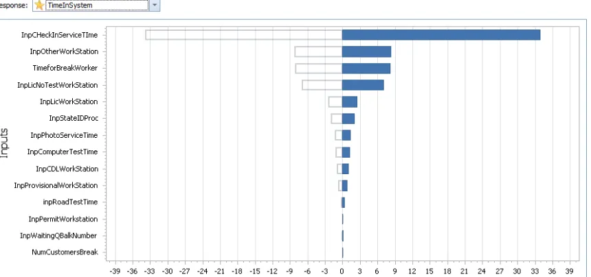
Figure 4.1 Sensitivity of different inputs parameters on the output Lange (2015)127 Figure 4.2 Experiment overview . . . 129

Figure 4.3 Experimental sequence . . . 130

Figure 4.4 Column correlation K-NOLHD and SLHD DMV dataset . . . 131

Figure 4.5 Responses histograms for K-NOLHD and SLHD experiments DMV dataset . . . 133

Figure 4.6 MSPE - constant mean with separable and non-separable covariances139 Figure 4.7 MAX - constant mean with separable and non-separable covariances140 Figure 4.8 MSPE - Ada-Lasso mean with separable and non-separable covariances142 Figure 4.9 MAX - Ada-Lasso mean with separable and non-separable covariances143 Figure 4.10 Constant vs Ada-Lasso mean best results . . . 144

Figure 4.11 Effect of the number of replications on model accuracy - R2 _{. . . 145}

Figure 4.12 Effect of the number of replications on model accuracy . . . 146

Figure 4.13 All techniques comparison - R2 _{. . . 147}

(19)

(20)

ABBREVIATIONS

ABM Agent Based Modeling. 21

ALGP Adaptive-Lasso Gaussian Process. 97, 98, 100–102, 105–107, 110, 112, 117–120,

126, 143, 144, 149, 150, 153, 154, 159–161, 164

ALGPE Adaptive-LASSO Gaussian process with squared exponential covariance

func-tion. 107, 108, 116, 141, 142, 153, 159, 160, 164

ALGPM32 Adaptive-LASSO Gaussian process with Matèrn once differentiable

covari-ance function. 107, 108, 141

ALGPM32NS Adaptive-LASSO Gaussian process with Non-Separable Matèrn once

differentiable covariance function. 107, 108, 141

ALGPM52 Adaptive-LASSO Gaussian process with Matèrn twice differentiable

covari-ance function. 107

ALGPM52NS Adaptive-LASSO Gaussian process with Non-Separable Matèrn twice

differentiable covariance function. 108, 141, 142

ANN Artificial Neural Networks. 7

BLUP Best Linear Unbiased Predictor. 76

CART Classification and Regression Trees. 8

COSSO Component Selection and Smoothing Operator. 3

CRN Common Random Numbers. 15

CV Cross-validation. 39, 40, 42, 50, 66

DACE Design and Analysis of Computer Experiments. 12

DES Discrete Event Simulation. 2, 7, 14, 19, 21, 42, 120–125, 144, 154, 160, 163, 164

DOE Design of Experiments. 13, 84

GAMLSS Generalized Additive Models for Location, Scale and Shape. 7

(21)

GBRT Gradient Boosted Regression Trees. xiii, 17, 18, 32–35, 39, 50, 53–55, 57, 58, 66,

68–70, 72, 74–78, 80, 81, 102, 107, 110, 112, 116, 118–120, 124, 126, 137, 146–150, 153–155, 159–164

GP Gaussian Process. 2, 3, 5, 6, 8, 10, 11, 13, 15, 16, 18, 19, 39, 40, 43, 50, 52–55, 57, 59,

66–70, 72–78, 80, 81, 91, 92, 100, 101, 105, 106, 110, 112, 117–120, 123, 124, 129, 138, 142–149, 154, 155, 157, 158, 160, 162–164

GPCE Gaussian Process with constant intercept and squared exponential covariance.

51, 52, 59, 66, 138–140

GPCM32 Gaussian Process with constant intercept and Matèrn once differentiable

covariance. 51, 52, 59, 66, 67, 139

GPCM32NS Gaussian Process with constant intercept and Non-Separable Matèrn once

differentiable covariance. 50–52, 59, 66, 67, 77, 138–140

GPCM52 Gaussian Process with constant intercept and Matèrn twice differentiable

covariance. 59

GPCM52NS Gaussian Process with constant intercept and Non-Separable Matèrn twice

differentiable covariance. 51, 52, 59, 66, 138–140

GPQM32NS Gaussian Process with quadratic mean response and Non-Separable

Matèrn once differentiable covariance. 77

IDW Inverse Distance Weighting. 8

IE Industrial Engineering. 1, 2, 9, 13, 18, 42, 122, 162, 165

KED Kriging with External Drift. 11

LARS Least Angle Regression Selector. 87–89, 94

LASSO Least Absolute Shrinkage and Selection Operator. 85–91, 94

LHD Latin Hypercube Design. 6, 13, 14, 44, 60, 84, 132

MARS Multivariate Adaptive Regression Splines. 5, 6

MAX Maximum Absolute Error. 5, 18, 19, 21, 39, 43, 55, 67, 70, 73–76, 99, 100, 109,

110, 112, 118, 142, 144, 148, 159, 160, 162, 164

(22)

MLP Multilayer Perceptron. 3, 15, 16, 18, 25, 39, 53–55, 57, 59, 66, 68–70, 72, 74, 76,

77, 84, 100, 101, 105, 118, 124, 137, 146–148, 153–155, 157, 159–161, 163, 164

MLS Moving Least Squares. 8

MSPE Mean Squared Prediction Error. 9, 10, 14, 18, 21, 39, 43, 51–54, 67, 68, 73–80,

94, 98–100, 109, 110, 118, 124, 138, 141, 143–145, 147, 154, 159, 160, 162, 164

NOLHD Nearly Orthogonal Latin Hypercube Design. 13, 128–132, 137, 138, 141, 147,

149, 153, 154, 164

OK Ordinary Kriging. 8, 10–15

RBF Radial Basis Functions. 5, 6, 24, 56

REML Restricted Maximum Likelihood. 9, 10, 17

RF Random Forest. 3, 4, 6, 7, 15, 17, 18, 30, 32–34, 39, 53, 57–59, 76, 124, 137, 146, 147,

153, 161–163

RIDW Regression Inverse Distance Weighting. 8

RK Regression Kriging. 10–12

RMSPE Root Mean Squared Prediction Error. 5, 7, 19

RSM Response Surface Methodology. 3, 13, 91

SD Systems Dynamic. 2, 21, 42–44, 60, 73, 74, 77, 122, 164

SK Stochastic Kriging. 8, 12, 15

SLHD Sliced Latin Hypercube Design. 129, 131, 132, 137, 140, 141, 147, 150, 165

SVM Support Vector Machine. 3, 4, 6, 7, 15, 16, 18

SVR Support Vector Regression. 22, 24, 25, 39, 53, 56–58, 76, 121

UK Universal Kriging. 11, 13, 14

UML Unified Modeling Language. 92

(23)

Chapter 1 Metamodeling in Engineering

1.1 Introduction

A simulation is an abstraction of reality used to provide a simplified representation of our perception of the salient features of a system, which in most cases, is complex and nonlinear. Large simulations are still very time consuming and expensive to run; thus, when the dimensionality of the problem gets large, it is not recommended that the simulation model be used to perform sensitivity analysis or optimization. To overcome this problem the analyst has to employ another level of abstraction and build a metamodel, which provides faster execution and better comprehension of the simulated system. The metamodel provides (ideally) a sort of “gray-box” for the I/O relationships; however, the ability of the metamodel to predict reality depends completely upon the accuracy of the simulation models. Once fitted, a metamodel can be used for several purposes 1) model approximation, 2) model exploration, 3) problem formulation, 4) global or multi-objective optimization, etc. (Wang and Shan, 2007).

The main objectives of this dissertation are:

(24)

separable covariance functions on the prediction performance of Gaussian Process (GP) will be tested (GP is the currently most-used technique in engineering), which

is generally overlooked in simulation metamodeling.

• Propose an improvement in how to incorporate more information into the non-stationary trend component of a Gaussian process to metamodel simulations with a large number of parameters. The effect of loose coupling of modern covariate selection techniques with GP will be studied with the aim of improving the predictive performance of GP applied to deterministic and stochastic simulation.

• Contribute to metamodeling applications in the field of IE by applying metamodeling to two different simulation paradigms, namely, Systems Dynamic (SD) and Discrete Event Simulation (DES). First, the efforts are focused on comparing different metamodeling techniques applied to two SD hospital simulations done to determine the most accurate metamodels when responses are highly non-linear and their distributions non-normal. Second, study the impact of stochastic simulation on different metamodeling approaches using a DES of the Division of Motor Vehicles of NC.

1.2 Literature Review in Simulation Metamodeling

In this section different metamodeling methods applied to engineering problems are explored. An effort has been made to separate non-GP1 _{techniques from GP models.}

(25)

1.2.1 Non-Gaussian Processes Metamodels

The main idea behind metamodeling is to approximate a complex system with a simple, parametric or nonparametric, and less computationally expensive method to explore how a set of covariates are related to one or more response variables. The work of Box and Wilson (1951) introduced the concept of Response Surface Methodology (RSM) and the use of low order polynomials to approximate the underlying relationship among variables (Box and Draper, 1987) . This section reviews different modern metamodeling techniques

applied to simulation in engineering.

(26)

better because of their interpolation properties, but when the number of samples get large machine learning methods such as SVM, RF and Radial Basis functions produce better results. With regard to execution time the authors pointed out that Random Forest provides the best compromise of speed and accuracy.

Can and Heavey (2012) compared Genetic Programming, which has the capability to evolve programs using symbolic regression, and Artificial Neural Networks as metamodel-ing techniques for three Industrial Engineermetamodel-ing problems 1) Automated Material Handlmetamodel-ing System (Kuo et al., 2007), 2) the (s, S) Inventory Control System (Biles et al., 2007), and 3) Production Line (Papadopolous et al., 1993). The main evaluation criteria were (i) training and test performance and (ii) computational effort. Their conclusions were that Genetic Programming showed a better performance in out-of-sample prediction; however, its main drawback was that it is more expensive to fit even considering the tuning time Artificial Neural Networks require to avoid over-fitting.

(27)

validation, pointing out that the popular leave-one-out cross-validation does not convey the information needed to assert metamodel accuracy; instead, leave-k-out cross-validation must be used and a good rule of thumb for k is k = 0.1N or k = √N, where N is the sample size (Wang and Shan, 2007, p. 12). In regard to the evaluation criteria, the authors used the three most common validation methods, presented below:

RM SP E =

s PN

i=1(yi−yˆi) 2

N (1.1)

M AX = max_|yi−yˆi|, i= 1, . . . , N (1.2)

R2 = 1₋

PN

i=1(yi−yˆi) 2

PN

i=1(yi−y¯)

2 (1.3)

The Root Mean Squared Prediction Error (RMSPE) is a measurement used to evaluate general accuracy; while, the Maximum Absolute Error (MAX) gives information about local accuracy and R2 _{provides spatial proximity between the answers produced by the}

simulation model and the metamodel.

Jin, Chen, and Simpson (2001) compared Second Order Polynomial Regression, Mul-tivariate Adaptive Regression Splines (MARS), Radial Basis Functions (RBF) and GP with Gaussian Correlation. Their evaluation criteria were accuracy, efficiency, robustness, transparency and simplicity. They evaluated 14 test problems classified according to three features: 1) problem scale, which is given by the number of covariates, 2) nonlinearity, defined as an R2 _≤ ₀_.₉₉ _{when a low order polynomial model is fitted, and 3)} _{noisy vs}

smooth surface. They concluded that MARS, RBF, and GP with Gaussian correlation

(28)

is the most suitable model. Finally, they pointed out that for small sample sizes RBF outperforms the other methods and that GP was the least efficient when fitting time was considered.

Li et al. (2010) compared RBF (Gaussian function with Ridge regularization), SVM with Gaussian kernel function, Neural networks, GP with Gaussian correlation and un-known constant, and MARS. The test bed was comprised of 16 stochastic problems (functions with added noise). They divided the data into training, validation and testing sets, but no cross-validation was performed. They used the average value of the repeated runs of the model to develop the metamodel and Latin Hypercube Design (LHD) to gener-ate the designs. The evaluation criteria were accuracy, robustness (the algorithm does not deteriorate when tested on different data), and efficiency. Li et al. (2010) concluded that SVM provided the best compromise of accuracy and robustness, but for more complicated models (higher dimensionality and heterogeneous errors) RBF was more efficient. They also pointed out the importance of interpretability, stating that only MARS has a simple interpretation and all the remaining methods, although they are accurate and robust, are difficult to interpret based on the underlying relationships among the input covariates and the response.

(29)

even though Boosting and SVM have better performance than RF, SVM was a much more expensive procedure. Finally, they pointed out the ability of RF and Boosting to find simpler, faster, and more interpretable (the understandability of why the model is true or how it is induced from the data) models (Ogutu, Piepho, and Schulz-Streeck, 2011, p. 8).

Boutselis and Ringrose (2013) compared Artificial Neural Networks (ANN) and Generalized Additive Models for Location, Scale and Shape (GAMLSS) as potential metamodeling techniques applied to computer combat simulation. They stated that when the relationship between variables is too complicated to be predefined parametrically, the flexible methods of ANN and GAMLSS could be used. Regarding GAMLSS they said, “[I]t is a very flexible approach to modeling not just the mean but also the vari-ance, skewness and kurtosis of the response variable using flexible (e.g. spline) models” (Boutselis and Ringrose, 2013, p. 6088). The authors used RMSPE as the key indicator of out-of-sample prediction. They concluded that both methods produce quite similar out-of-sample prediction performance, with GAMLSS more accurate for skewed data; in addition, GAMLSS requires more involvement in model development and selection which could be useful in understanding of the data and the results.

Hsieh, Chang, and Chien (2014) proposed a response surface method built on a second order polynomial to capture the relationship between the cycle time of normal lots and the percentage of hot lots in semiconductor manufacturing. Their model consisted of a DES experimented by a simplex lattice design. Then, a second order polynomial was fitted and if the resulting model was not satisfactory (based on R2_{) more points were}

(30)

reliable and easy-to-use analytical model.

Salemi, Nelson, and Staum (2014) studied the applicability of Moving Least Squares (MLS) regression with anisotropic weight function for high-dimensional stochastic

sim-ulation. They compared MLS, Classification and Regression Trees (CART), Stochastic Kriging (SK) with Gaussian correlation, Weighted Least Squares (WLS) regression. They reported that MLS produced results even when the sample size was larger than 5,000; whereas SK and WLS were unable to obtain a result for that sample size since the computer ran out of memory. They concluded that their MLS outperformed the other methods forecasting the M/G/1 queue with 5, 25, and 75 dimensions.

Joseph and Kang (2011) demonstrated that the Inverse Distance Weighting (IDW) interpolation method can be significantly improved when coupled with a linear regression method. Their work was focused on reducing the computational burden of GP methods, while maintaining prediction accuracy. The proposed Regression Inverse Distance Weight-ing (RIDW) consists of fittWeight-ing a penalized regression model to obtain a sparse global trend approximation of the response; then, the residuals are used for interpolation based on a modified IDW that allows for anisotropy (different importance for each covariate) and truncated neighborhood (include just a specific number of points around a new prediction site). They compared RIDW with Ordinary Kriging (OK), concluding that the former has comparable prediction accuracy to the latter, but requires less computational effort (there is no need to invert the correlation matrix). Finally, they justify their use of global

(31)

1.2.2 Gaussian Process Metamodeling

In this subsection some relevant work in Kriging literature is presented. Firstly, a review of works outside IE is given. Secondly, the most relevant works in the IE field are summarized.

1.2.2.1 Some applications outside Industrial Engineering

Kriging is a general technique used for interpolation that originated in the field of Geo-statistics (Kbiob, 1951; Matheron, 1963). Its applications span a wide range of fields from geology and agriculture to economics and engineering. The following is a broad overview of the current practice outside engineering.

Mardia (2007) pointed out that the method of Maximum Likelihood (ML) used in computer experiments compares favorably to the use of variograms -the current practice in geostatistics- allowing the integrated estimation of the mean response vector and the covariance hyper-parameters. However, he also stated that the ML method is computa-tionally demanding for two reasons: the matrix factorization and the multidimensional optimization of the autocorrelation parameters. He also said that ML should be preferred over Restricted Maximum Likelihood (REML) because the latter is more sensitive to the effect of the mean response having higher Mean Squared Prediction Error (MSPE) in some cases. Pollice and Bilancia (2002) studied Kriging as a linear mixed effect model comprised of a mean part, a spatially correlated component, and random noise. They mention that the use of fixed mean effect and REML produces biased covariance estimates in an application to the prediction of soil properties.

(32)

small samples but high-dimensional inputs. They explained that the autocorrelation func-tion weights are governed not only by the trend specificafunc-tion -ranging from linear models to Fourier series- but also the choice of autocorrelation function; the Gaussian covariance is generally preferred because of its simplicity and symmetric properties. Moreover, Gins-bourger et al. (2009) noted that Kriging with a constant, also known as OK, is the most commonly used version of Kriging, but it has some flaws when the response is highly non-linear. They studied the effect of linear and quadratic mean responses, noticing that they produced poor results for extrapolation. Finally, they tested a non-linear additive model for the trend and ML for Kriging the residuals, but the resulting MSPE did not improve as expected.

Bachoc et al. (2014) applied Kriging to a thermal-hydraulic system. Their main goal was to improve model prediction by conditioning the mean response and the autocor-relation function through the use of priors. They reported the use of cross-validation to validate their results and used different autocorrelation functions, namely, Gaussian, Exponential, and Matèrn, once and twice differentiable in their separable form. They concluded that the use of a two stage Gaussian process model, whose first stage computes the autocorrelation function of the residuals using REML and then the second recalibrates the mean response, produced better mean squared prediction error than the regular GP.

(33)

dimension to be included in the model, while other authors have set the minimum at

2p+ 20 where p represents the number of predictors. Finally, they concluded that using RK the analyst can get “the best” of the data and that the “logit transformation” applied to the response variable can be useful to model non-linear relationships (Hengl, Heuvelink, and Stein, 2003).

Hung (2011) proposed the Iterative Reweighted Least Angle Regression (IRLARS) algorithm for Gaussian Processes and presents an application for circuit simulations. The method first computes adaptive Lasso (Least Absolute Shrinkage and Selection Operator) which perform simultaneous estimation and variable selection and then GP, repeating that sequence until convergence. The main drawback of his method is that it is iterative, which means the optimization process has to be run several times to achieve convergence. This becomes intractable for large GP models, and get worse if cross-validation and several random starting points are needed.

(34)

Finally, including a trend component allows for a broader interpretation of the Gaus-sian process because the analyst can have separate information about the underlying interpolation components. Despite the broad utilization of RK in geostatistics, the method has not extended through computer experiments, where the general trend is OK or its heteroskedastic version SK. A detailed explanation of this method and other advanced topics in the field of spatial statistics can be found in Cressie (2015), Illian et al. (2008), Isaaks and Srivastava (1989) and Gelfand et al. (2010).

1.2.2.2 Kriging in Engineering

The application of Kriging to engineering problems started with the work of Sacks et al. (1989). Later, Lophaven, Nielsen, and Sondergaard (2002) implemented the Design and

Analysis of Computer Experiments (DACE) using Matlab, making it a popular tool for

Kriging metamodeling. The implementation consists of efficient computations based on Cholesky decomposition for the autocorrelation matrix and LU transformations for the mean response, making it the cornerstone for newer Gaussian process software (Pedregosa et al., 2011; Couckuyt, Dhaene, and Demeester, 2014). An implementation of DACE using

object oriented paradigm in Matlab was provided by Couckuyt, Dhaene, and Demeester

(2014), extending the number of autocorrelation functions available to include the Matèrn family in its separable form. In this dissertation we use thesklearnGaussian process class

available in Python (Rossum, 1995) that according to its authors is a “shameless copy”

of the original DACE (Pedregosa et al., 2011). The interested reader can see Roustant, Ginsbourger, and Deville (2012, p. 3) for a detailed analysis of the current implementations

inR andMatlab. In summary, keeping track of the available software to fit Kriging models

(35)

and also define the availability for general use because R and Python are free but Matlab

is commercial.

Kleijnen et al. (2015) reviewed how RSM and Kriging relate to different Design of Experiments (DOE). They emphasized that each metamodel defines a specific DOE which is more appropriate for sensitivity analysis and optimization. They related fractional

fractorial designs with different resolutions and central composite design with RSM and

LHD or Nearly Orthogonal Latin Hypercube Design (NOLHD) with Kriging methods; additionally, they propose that the analyst should usesequential bifurcation to identify the most important parameters. They gave a detailed explanation of OK and UK applied to both deterministic (homoskedastic error) or stochastic (heteroskedastic error) simulation. Finally, the author made a statement that reflects most of the applications of Kriging in IE: “The disadvantage of UK is that UK requires the estimation of additional parameters:

beside µ=β0. We conjecture that the estimation of these q−1 extra parameters explains why UK has a higher MSE. In practice, most Kriging models do not use UK but OK”

(Kleijnen et al., 2015, p. 20).

(36)

optimization. They experimented with a small (s,S) inventory example using LHD and OK with Gaussian correlation function.

Mehdad and Kleijnen (2014) proposed a variant of Kriging known as Intrinsic Kriging (IK) which is based on the idea of using integrated random functions as means of filtering trend, equivalent to an integrated process in time series. They compared IK versus OK and UK with a fixed order polynomial of degreep(homoskedastic and heteroskedastic versions) concluding that IK gives smaller MSPE than OK and UK but requires more work selecting covariance parameters. Kleijnen (2009) provided an introduction to Kriging for the field of simulation and discussed the use of LHD and sequential design for simulation experiments taking advantage of the Gaussian process variance at non-simulated points. He explained both deterministic and stochastic Kriging framed as OK formulas. Some of his conclusions were: 1) Kriging studies need to be carried on more realistic simulations that the classical

M/M/1 queuing and the (s, S) inventory model which are simple academic examples,

and 2) more studies are required to fill the gap between Kriging and simulations with multivariate output. Dellino (2007) proposed a robust optimization framework which combines Taguchi methods and Kriging, but the main drawback is that the entire work is supported by only two examples based on the Economic Order Quantity (EOQ) and the (s,S) inventory problem making the results difficult to generalize to larger simulations.

Ankenman, Nelson, and Staum (2010) introduced the concept of Stochastic Kriging

(37)

‘heteroskedastic nugget effect’. They demonstrated that using this additional information provided by the replications, the analyst can get a more accurate model than deterministic

OK. Staum (2009) presented examples for the application of SK to the M/M/1problem

and explained why it is important to consider the effect of local variability produced in stochastic modeling. Moreover, he emphasized that misspecification of the regression basis produces poor predictions justifying the use of SK with just a intercept term for the mean and relaying mostly in the interpolation power of the random part. Chen, Ankenman, and Nelson (2013) showed how incorporating gradient information improves surface prediction. Additionally, Chen, Ankenman, and Nelson (2012) study the effect of Common Random Numbers (CRN), concluding that when the aim of the metamodel is to provide accurate prediction values as in financial risk, CRN is not recommended. However, CRN are recommended when better parameter estimates are required for sensitivity analysis.

Finally, the interested reader is encouraged to see Rasmussen and Bro (2012) and Rasmussen (2006) for a full treatment of Gaussian processes, and Santner, Williams, and Notz (2013), Fang, Li, and Sudjianto (2005), and Sacks et al. (1989) for applications of Kriging in computer experiments.

1.3 Discussion

(38)

not seem to be popular in other engineering fields. Table 10.1 in Hastie et al. (2009, p. 351) presents the most popular “off-the-shelf” data mining techniques. They pointed out that SVM and MLP on the one hand have good predictive power and can handle linear combination of covariates but, on the other hand, have bad scalability for large samples and poor interpretability, being extremely sensitive to input transformations. Even though they did not consider GP in the table, it can be said that GP closely follows SVM and MLP characteristics.

Table 1.1: Most cited metamodeling techniques

Technique Study

SVR

Villa-Vialaneix et al. (2012)

Ogutu, Piepho, and Schulz-Streeck (2011) Li et al. (2010)

Wang and Shan (2007)

Jin, Chen, and Simpson (2001)

MLP

Boutselis and Ringrose (2013) Villa-Vialaneix et al. (2012) Can and Heavey (2012) Li et al. (2010)

RF Villa-Vialaneix et al. (2012)

Ogutu, Piepho, and Schulz-Streeck (2011)

GP

Salemi, Nelson, and Staum (2014) Villa-Vialaneix et al. (2012) Joseph and Kang (2011) Li et al. (2010)

(39)

In regard to methods based on Trees, Hastie et al. (2009) say that their advantages are scalability, robustness to input transformation, and mixing different types of data. The main disadvantages are poor predictive power and difficulty of extracting linear com-binations; additionally, they give a “fair” interpretability score to trees. It is important to point that RF and GBRT are the strongest tree-based techniques and according to Hastie (2014) they have better prediction performance than most of the tree-based methods. He

also said that in general GBRT should perform better than RF.

Finally, Table 1.2 presents the current Gaussian process standard practices in both

spatial statistics and computer experiments. Outside of engineering the practice is to

detrend the surface using low-order polynomials and then compute the covariance structure either using variograms (the preferred choice) or REML to the detrended errors. On the other hand, computer experiments use a flat mean response and relies on an anisotropic parameter search to estimate the covariance structure in an integrated way with the mean response using ML.

Table 1.2: Current Gaussian process practices in Spatial Statistics and Computer Experiments

Area Mean response Covariance Separability θparameters

Spatial Statistics Polynomial function Matèrn No Variogram, RMLE

(40)

1.4 Dissertation Outline

Based on the previous review, we observed a lack of an integrated comparison of the state-of-the-art techniques with applications to simulation problems. Moreover, an im-portant number of the comparisons were done with either artificial data or data that is not representative of the behavior of complex simulated systems found in the IE models. Another important issue addressed by this work is the comparison between separable (product of one dimensional correlations) and non-separable (geometrically anisotropic) correlation functions Additionally, more importance should be given to the mean response when using Gaussian processes in computer experiments, especially for high-dimensional problems, so studying its importance for both deterministic and stochastic simulation will be an important part of this work.

The remainder of this dissertation is organized as follows:

• Chapter 2 presents a state-of-the-art comparison of current machine learning al-gorithms, namely, GP, SVM, MLP, RF and GBRT. Two different simulations are analyzed using three criteria: MSPE, R2_{, and MAX. Special emphasis is given to}

reproducible research providing all the information needed to replicate the results presented. In order to assess the quality of MSPE,R2 _{and MAX, cross-validation is}

used. Another important issue addressed in this chapter is the interpretability of each technique, which is generally overlooked in engineering applications.

• Chapter 3 studies the effect of different specifications of trend functions in GP. A two-stage method is proposed coupling GLMNET, the state-of-the-art model selection

(41)

adequate specification of the global trend for both prediction accuracy and model interpretation. The results from this chapter are contrasted with those obtained

in Chapter 2 following the same criteria RMSPE, R2 _{and MAX and degree of}

interpretability.

• Chapter 4 explores the effect of the loose coupling proposed in Chapter 3 on a stochastic simulation. A DES of a DMV office in Charlotte, North Carolina is metamodeled in order to determine how the modern machine learning techniques respond to simulations with noise due to replications. Two experimental designs are analyzed conjointly with the proposed techniques in order to determine how sensitive the techniques are to the locations of points in the experimental region. The effect that the number of replications per point has on the accuracy of the responses when using GP is also explored. Finally, a complete analysis of coverage is presented.

(42)

Chapter 2 Metamodeling: A State-of-the-Art

Com-parison

2.1 Introduction

In this dissertation the variable definitions used in Hastie et al., 2009 will be employed. An input variable is given byX, whose components are _{Xj}p1, wherepis the total number of

features. A quantitative output is given by Y. Sample values xi are written in lowercase, where xi is theith observed value ofX. Bold uppercase letters represent matrices. The set of samples, e.g. {xi}N1 would be theN ×p matrixX. Vectors withN elements are bold;

thus y and xj represent all observation on the response and the Xj variable respectively. Finally, xT

i is the transpose of xi since all vectors are assumed to be column vectors and

xi is the ith row of X.

(43)

To date, there are three major paradigms in simulation: SD, DES, and Agent Based Modeling (ABM). SD is a high level abstraction technique that models the dynamics of the systems defining accumulators (stocks) and flow rates (flows) that are connected by feedback loops. DES has a lower level of abstraction since it mirrors the process the modeler observes in real life; thus, it is a process-oriented technique that focus on modeling the sequence of operations done with entities. Finally, ABM is a bottom-up approach used when there is information about how the individual elements of a system behave, but no general understanding of how the general process behaves (Borshchev, 2013).

In one way or another, all these techniques, regardless of their abstractions, can still be very complicated and time consuming to analyze. To handle this problem another level of abstraction called “metamodel” (a model of the simulation) is used in place of the simulation to mimic the responses Y observed in the real world. Because the metamodel is a simplification of the simulation it adds additional noise m, so the real world response can be approximated by Y =fˆˆ(X) +sim+m.

(44)

2.2 Modern Machine Learning Techniques

Modern machine learning methods have overtaken simple linear models because of their better prediction accuracy when the relationship between the covariates and the response are non-linear, cannot be defined or both (Breiman et al., 2001). In this section a general overview of the five methods used in this chapter is given. For a complete and detailed derivation of each method the interested reader is encouraged to see Hastie et al. (2009) and Bishop (2006) who provide a deeper overview of each model.

2.2.1 Support Vector Regression (SVR)

Introduced by Cortes and Vapnik (1995) theε-SV regression finds a functionf(x)that has at mostε deviation from all training pointsyi; no deviation larger thanε will be accepted. Let Equation 2.1 be the function that approximates the relationship of the covariates and the response, where φ(_·) represents a feature mapping to a higher dimension e.g.

xT _{= (}_x

1, x2)−→φ(x)T = (x1, x2, x21, x1x2, x22)

f(x) = β0+φ(x)Tβ (2.1)

Under Support Vector Regression (SVR) the optimal parameters for β0 and β are

found by minimizing Equation 2.2, whereC is a tuning parameter to control the trade-off between flatness off(_·)and the amount of error above to be tolerated. This condition is needed because most of the time it is not possible to approximate all responses within

precision (Smola and Schölkopf, 2004, p. 200). λ is a penalty parameter applied to the

(45)

Equation 2.3 is the -insensitive loss function that ignores errors smaller than. Basak, Pal, and Patranabis (2007), Smola and Schölkopf (2004), and Hastie et al. (2009) show the step-by-step procedure for solving the dual optimization problem of Equation 2.2.

H(β, β0) = C

N

X

i=1

V(yi, f(xi)) +

λ

2||β||

2 _(2.2)

where

V(yi, f(xi)) =

  

 

|f(xi)−yi| − if |f(xi)−yi| ≥

0 otherwise

(2.3)

They also show the optimal solution is given by Equations 2.4 and 2.5.

ˆ

β=

N

X

i=1

(ˆα_i∗₋αˆi)φ(xi) (2.4)

ˆ

f(x) = N

X

i=1

(ˆα_i∗₋αˆi)hφ(x), φ(xi)i+β0

ˆ

f(x) = N

X

i=1

(ˆα_i∗₋αˆi)k(xi, x) +β0 (2.5)

The important tuning parameters are C, ε and the type of kernel k(_·,_·). A kernel is essentially a covariance function that is symmetric and positive definite, and maps from input to feature space (Genton, 2002). In this work we follow Cherkassky and Ma (2004) who proposed an automatic hyper-parameter estimation from the data, reducing

(46)

that, according to the authors, includes the effects of outliers in the data.

C = max (_|y¯+ 3σy|,|y¯−3σy|) (2.6)

For computingthe author proposed Equation 2.7 which requires the estimation of two additional parameters τ and σ. According to his experiments τ = 3 was a robust choice for different datasets. They proposed to estimateσ from the data using the residuals of a

high-order polynomial as shown in Equation 2.8, where N represents the total number of

training samples and pthe number of covariates being estimated, and yˆare the predicted values from a high-order polynomial (second-order in our case).

=τ σ

r

ln(N)

N (2.7)

ˆ

σ2 = N

N ₋p

PN

i=1(yi−yˆi)2

N

!

(2.8)

In addition,linear,RBF, andsecond and third-order polynomial kernels are used based on the fact that the linear kernel is less prone to over-fitting in high-dimensions, but less flexible when the relationship between the regressors and the response is non-linearly separable; whereas, RBF and polynomial kernels exhibit the opposite behavior. Equation 2.9 shows the RBF kernel for any two inputs x and z, where γ = 1/2σ2_{. Finally, it is}

important to mention that Hastie et al. (2009) showed that SVR can be heavily affected bythe curse of dimensionality and noisy factors.

(47)

In summary, the hyperparemeters used in SVR were optimized testing different values for: kernel, gamma, C, epsilon and degree.

2.2.2 Multilayer Perceptron (MLP)

A sketch of a MLP is given in Figure 2.1 which illustrates the classic topology of a

feedforward artificial neural network (Svozil, Kvasnicka, and Pospichal, 1997). The input

layer has one node for each of the features in the design matrix and communicates the

external variables to the network. Then, the network shows a set of hidden layers, each comprised by a set of nodes. The number ofhidden layers and their respective nodes must be tuned by the user because incorrect specification of these parameters can induce either under or overfitting. Finally, the output layer consists of just one node for regression problems that uses a linear transfer function (Karsoliya, 2012).

...

... ...

X1

X2

X3

X16

H1,1

H1,8

H2,1

H2,8

Y7

Input layer

1st _Hidden layer

2nd _Hidden layer

Ouput layer

(48)

In general, one or two hidden layers with the same number of nodes are recommended by Karsoliya (2012, p. 716). In regard to the number of nodes per hidden layer, several rules of thumb are available in Karsoliya (2012, p. 716) such as the total number of nodes should be less than twice the number of nodes in the input layer, the number of nodes should be between the number of inputs and outputs nodes, etc. We used Equation 2.10 to determine the number of hidden nodes (Nh). Ni andNo represents the number of input and output nodes respectively,Ns the number of samples in the training set, and k is a scaling factor between two and ten.

Nh =

Ns

k(Ni +No) (2.10)

Another important parameter that is predefined by the user is the transfer function used to induce non-linearity to fit more complex functions. The logistic sigmoid and the

rectifier linear unit are the most commonly used, the later being more popular nowadays

(LeCun, Bengio, and Hinton, 2015; Nair and Hinton, 2010). The functional forms are given in Table 2.1.

Table 2.1: Transfer functions

Name Formula

Rectifier linear unit (Relu) f(x) = log(1 +ex₎

Sigmoid (logistic) f(x) = ₁₊1_ex

(49)

scaling” method where t denotes time. Next, the initial learning rate must be set to a small number in the interval [0,1]. Modern software allows forL2 regularization in order to

control over-fitting (see the MLP object in Pedregosa et al., 2011, for a detailed example).

X2 w2

Σ

f

Activate function

Z Output

X1 w1

X3 w3

Weights

Bias

w0

Inputs

Figure 2.2: Weight and activation function

(50)

by Equation 2.13.

ηj = p

X

i=1

wIiXi+wI0 (2.11)

f(ηj) =log(1 +eηj) (2.12)

Y =

m

X

j=1

wHjf(ηj) +wH0 +ε (2.13)

The main parameters to tune are the number of hidden layers and the number of nodes associated with each one, the transfer function, the initial learning rate values and its behavior during the training, and the regularization parameter. Once the feed forward pass has reached Equation 2.13 the prediction error is computed and if the convergence criterion is not met, the error is back-propagated in order to update thew. This process continues until convergence.

For hyperparameters optimization the following parameters were evaluated: hidden_-layer_sizes, activation_function, alpha, learning_rate, learning_rate_init.

2.2.3 Random Forest Regression (RF)

The Random forest is an ensemble method introduced by Breiman (2001). In simple words, the approach consists of an ensemble of several regression trees (as described in Breiman et al., 1984) which obtains a prediction based on a unitary vote from each tree. In order to understand the idea of RF first it is important to explain what a tree is. Figure 2.3 depicts different views of a regression tree. On the left can be seen a basic binary tree structure that consists of a set of if-then-else statements, that starting from a root

(51)

x13 >= 18

x13 >= 22

x13 >= 32

x5 < 124 x5 < 99

x5 < 124

x5 < 101

x13 >= 14

x5 < 70

x13 >= 14

x5 < 125 6.1

7.8 16 9.3

19 29 9.4 21 30 28 47 52 yes no (a) Tree x5 x13

(b) 3D surface

x5

x13

60 80 100 120 140

20

30

40

50

(c) 3D surface

Figure 2.3: Regression Tree for response 4 Hospital 1 data

The algorithm generates {Rm}M1 piece-wise constant regions of the feature space and

the predicted value in each region is the average response of the observations at that region _fˆ₍_x_{) =} PM

i=1y¯mI(x ∈ Rm) where Rm is an hypercube region, y¯m the average

of the responses in the region and I is the indicator function that is 1 if x is in Rm, zero otherwise. At each iteration the algorithm minimizes the node impurity, which in the case of regression is given by e(T) = PN

i=1

h

yi−PMm=1y¯mI(x∈Rm)

i2

finding at each iteration the variable/split combination that minimizes the prediction error e(T) with respect to y¯m and Rm. Once the algorithm has converged it gives a piece-wise con-stant model that is easy to interpret (a good read is Loh, 2011) as depicted in Figure 2.3(a).

(52)

either the data or the response, 3) they are sensitive to small perturbations having an impact on out-of-sample predictions and 4) its piece-wise constant structure affects prediction accuracy when the response decays smoothly.

In order to overcome these flaws Breiman (2001) proposed an ensemble of trees -a forest- that using some randomization strategies produces a more accurate and smooth surface than a single tree. The general description of how to generate a RF is presented in Algorithm 1, below:

Algorithm 1 Random forest pseudo-code

1: for m= 1 toM do .M is the total number of trees

.Sample with replacement N samples from X

2: X_m ←bootstrap_N(X)

3: Fit a random forest tree T_m(X_m) following these instructions for each terminal

node

4: while Minimum node size is not reached do

5: Randomly selectd out of p features

6: Find the best feature\split combination out of the dreduced set.

7: Generate a binary partition of the feature at the split point

8: end while

9: end for

10: return the ensemble _{Tm(Θm)}Mi

The recursive procedure used to fit a random tree using N bootstrapped observations and just m features at each iteration produces more uncorrelated trees which, according to Breiman (2001), improves the variance. The prediction of a random forest is the simple average of the unitary vote of the prediction of each tree in the random_forest as seen

(53)

if-then-elserules for the bth tree, B is the total number of trees andxis a new sample.

ˆ

frfM(x) = 1

M

X

m=1

T(x: Θm) (2.14)

Algorithm 1 is efficiently implemented in Pedregosa et al. (2011). Hyperparameter opti-mization was experimented on: max_features, max_depth, min_samples_split, min_-samples_leaf, and n_estimators options.

x13 >= 20

x13 >= 28

x5 < 122

x13 >= 23

x5 < 72

x5 < 127

x13 >= 14

x5 < 101 6.4

8.7

17 30

12

26

29 53

49

yes no

x13 >= 20

x13 >= 30

x5 < 122

x13 >= 24

x5 < 99

x13 >= 14

x5 < 127 6.8

8.9

18 32

15

28 43

61

yes no

(a) Boostrapped trees

x5

x13

(b) 3D surface

Figure 2.4: Random Forest for response 4 Hospital 1 data

2.2.4 Gradient Boosted Regression Tree (GBRT)

(54)

base learner) to the residual at each iteration.

F(x) = M

X

m=0

βmb(x; Θm) (2.15)

When the base learner is a regression tree, each iteration of GB grows a new tree. The process improves the fitting in regions where the previous trees did not do well. This is achieved because the new tree is fit to the “pseudo” residuals (the error left from the previous fits), generating completely different trees from iteration to iteration as shown in the left plot in Figure 2.5. In general, the trees will not be as deep as RF because the latter needs bushy trees, namely trees with high level interactions, to reduce variance through averaging. The right plot in Figure 2.5 shows that after sequentially fitting shallow trees GBRT produces a smoother surface-response than a simple regression tree (Figure 2.3)

x13 >= 18 x13 >= 22

x13 >= 32 x5 < 124

x5 < 99 x5 < 124

x5 < 101 x13 >= 14 x5 < 70

x13 >= 14 x5 < 125

6.1 7.8 16 9.3 19 29 9.4 21 30 28 47 52

yes no x13 < 12

x5 < 84 x13 >= 14 x13 < 16

x13 >= 20 x5 >= 134

x5 < 135 x5 < 98 x5 >= 101

x5 < 130 x5 >= 102

-5.8

-0.82

-4

-8.5 -0.58 -1.4

0.66 6

-0.81 6.8 13 9.4

yes no

(a) Sequential trees

x5

x13

(b) 3D surface

Figure 2.5: Random Forest for response 4 Hospital 1 data

(55)

Algorithm 2 Generalized Boosting

1: Initialize the functionF₀(x) = 0

2: for m= 1 toM do

3: β_m,Θ_m ←arg min

β,Θ

PN

i=1L(yi−Fm−1(xi) +β b(xi : Θ))

4: F_m(x)←F_m−1+εβmb(x: Θm)

5: end for

6: return fˆ(x) =FM(x)

linear regression or trees. The process needs an initial value for the function Fo(x), and then sequentially fits the base learner to the residuals. The Generalized Boosting algorithm uses astage-wise procedure to compute the parameters βm andΘm in line 3 of Algorithm 2 (Friedman, 2002; Hastie et al., 2009). According to Friedman (2002) this stage-wise procedure makes tractable a potentially difficult problem, an idea that will be explored in Chapter 3. Line 4 shows the update of the cumulative sequential fitting, whereε is a scalar in the range(0,1] used to slow down the rate of overfitting, by updating the model by a small amount.

A customized implementation of GB for trees is given in Friedman (2002) Algorithm 1, which is presented here in Algorithm 3. The modification for trees starts in Line 6

where GBRT fits a L-terminal nodes tree that produces _{Rlm_}L

1 disjoint regions. As

explained before, a regression tree predicts a constant value for each region; thus, the update after each iteration just reduces to an estimate a “location” parameter for each region of the mth tree as in Line 8 and then adds it to the cumulative model using the indicator function as in Line 10 (Friedman, 2002). The interested reader is encouraged to read Friedman (2002, p. 2).

Simulation Metamodeling with Gaussian Process: A Numerical Study.

ABSTRACT

DEDICATION

BIOGRAPHY

ACKNOWLEDGEMENTS

TABLE OF CONTENTS

LIST OF TABLES

LIST OF FIGURES

ABBREVIATIONS

Chapter 1

Metamodeling in Engineering

1.1

Introduction

1.2

Literature Review in Simulation Metamodeling

1.2.1

Non-Gaussian Processes Metamodels

1.2.2

Gaussian Process Metamodeling

1.3

Discussion

1.4

Dissertation Outline

Chapter 2

Metamodeling: A State-of-the-Art

Com-parison

2.1

Introduction

2.2

Modern Machine Learning Techniques

2.2.1

Support Vector Regression (SVR)

2.2.2

Multilayer Perceptron (MLP)

...

... ...

Σ

f

2.2.3

Random Forest Regression (RF)

2.2.4

Gradient Boosted Regression Tree (GBRT)