Abstract.
Diggs, Jonathan Andrew. Simulation of nitrogen and hydrology loading of forested fields in eastern North Carolina using DRAINMOD-N II. (under the direction of Dr. R. W. Skaggs and Dr. G. M. Chescheir)
A new version of DRAINMOD-N (DRAINMOD-N II) was used to evaluate the combined effects of soil variability, vegetation, drainage intensity, climate, and management practices on the hydrology and nitrogen (N) transport in forests. A better understanding of these processes will be useful in the development of management practices for reducing N loads from forests and in future large-scale modeling studies.
The objective of this study was to accurately model nitrogen loading at the field scale for three Coastal Plain forests in North Carolina using DRAINMOD-N II. Supporting objectives were to accurately model the hydrology of three forested fields using DRAINMOD, to determine litterfall and N uptake at the study sites, and to evaluate DRAINMOD and DRAINMOD-N II model accuracy by comparing predictions with measured values.
Water table elevations, drainage losses, and water quality were continuously measured at the study sites from 1995-2001. Soils on two of the fields were organic; the third field had a highly organic mineral soil. DRAINMOD was used to simulate the hydrology of the forested sites from 1995-2001. Very porous, highly organic soils made it difficult to determine
calculated from measurements of water table elevation and drainage outflow or from model calibration.
DRAINMOD-N II was used to predict cumulative N process rates and N losses in drainage. Litterfall production and N uptake inputs were determined using the forest productivity model PnET-CN. Michaelis-Menten input parameters for nitrification and denitrification in DRAINMOD-N II were determined by calibration. N mineralization was modeled as a function of organic matter (OM) content in the soil (initial OM and OM added by litterfall) and organic carbon decomposition rates.
DRAINMOD predicted water table elevations and drainage losses reasonably well when compared to observed data. Despite difficulties encountered in accurately determining the soil properties of the forest surface layers, and the hydrologic effect of maturing trees on evapotranspiration, the average absolute daily difference (AADD) of the water table depth predictions from 1995-2001 ranged from 13.0-28.4 cm, and the model efficiency, E, of the water table depth predictions ranged from 0.59-0.83. R2 values for the daily drainage rate predictions from 1996-2001 ranged from 0.69-0.85. Model efficiency (E), values for the daily drainage rate predictions from 1996-2001 ranged from 0.68-0.70. The normalized errors in cumulative drainage predictions from 1996-2001 ranged from -17.1 to 2.7 %.
1996-2001 ranged from -2.5 to 28.9 % for the three fields. Normalized errors in predicting
cumulative NH4-N loads for the 1996-2001 period ranged from -48.2 to 54.6 %. Normalized errors in predicting cumulative dissolved inorganic nitrogen (DIN) loads ranged from -6.4 to 23.9 %. The model was also calibrated using a six-year calibration for a better understanding of N transport processes and for use in future modeling studies.
SIMULATION OF
NITROGEN AND
HYDROLOGY
LOADING OF FORESTED FIELDS IN EASTERN NORTH
CAROLINA USING DRAINMOD-N II.
By
JONATHAN A. DIGGS
A thesis submitted to the Graduate Faculty of North Carolina State University
in partial fulfillment of the requirements for the Degree of
Master of Science
BIOLOGICAL AND AGRICULTURAL ENGINEERING DEPARTMENT
Raleigh 2004
APPROVED BY:
______________________________ _____________________________ Dr. R. Wayne Skaggs Dr. George M. Chescheir
Co-chair of Advisory Committee Co-chair of Advisory Committee
______________________________ Dr. H. Rooney Malcom
DEDICATION
To Mom and Dad - Thanks for everything. I love you both.
To JESUS CHRIST, nothing is possible without You.
I am the vine, you are the branches. If a man abides in me and I in him, he will bear much fruit; apart from me you can do nothing.
John 15:5
Thank You for loving me.
Just as the Father has loved me, I have also loved you. Abide in my love. John 15:9
Thank You for changing me.
BIOGRAPHY
Jonathan Andrew Diggs was born on August 10, 1979 in Newport News, Virginia to James and Sandy Diggs. He has two brothers, Greg and Michael. He grew up in Mathews County, Virginia on the Chesapeake Bay.
ACKNOWLEDGEMENTS
Many people were very helpful in doing this research, and without them this thesis would not have been written.
Thanks first of all to Dr. Skaggs for taking me on as a graduate student. I could not have asked for a better professor and advisor during my time here at NCSU. Dr. Skaggs sets an example for excellence in research and professionalism that I will not forget.
Thanks also to Dr. “Chip” Chescheir. Chip was always willing to drop whatever he was doing and take time to answer my questions, and I had many. He was always encouraging, and he helped me to think of problems from many different perspectives. I could not have completed my work without him.
Thanks to Dr. Mohamed Youssef for developing an excellent model and for helping me to learn how to use it. Dr. Youssef’s attention to detail and commitment to academic integrity were obvious, and it was a pleasure to get to know and work with him.
Thanks to Dr. Ge Sun for helping me with the PnET-CN model and to Wilson Huntley for helping me in the field.
TABLE OF CONTENTS
LIST OF TABLES viii
LIST OF FIGURES x
CHAPTER 1: INTRODUCTION 1
BACKGROUND 1
DRAINMOD-N II – MODEL DESCRIPTION 2
Nitrogen Cycle 3
Carbon Cycle 3
Modes of Operation 3
Governing Equation 4
Carbon and Nitrogen Transformations 5
Effect of Environmental Factors on C and N transformations 5 Application of Animal Waste and Crop Residues 7 Organic C Decomposition and N Mineralization/Immobilization 8
Nitrification 9
Denitrification 10
Plant Uptake 10
Atmospheric Deposition 11
Surface Runoff 11
MODEL TESTING 12
MODELING FORESTED CONDITIONS 13
OBJECTIVES 14
REFERENCES 16
CHAPTER 2: METHODS 18
SITE DESCRIPTION 18
Field – F3 18
Field – F5 18
Field – F6 18
HYDROLOGY MEASUREMENTS 19
Weather 19
Water Table 19
Flow 19
WATER QUALITY MEASUREMENTS 20
HYDROLOGY SIMULATIONS 21
Modeling Scenario 21
DRAINMOD Model Description 21
Infiltration 22
Surface Drainage 23
Subsurface Drainage 23
Evapotranspiration 23
Weather 24
Drainage System Parameters 25
Saturated Hydraulic Conductivity 25
Soil Water Characteristic 27
Upward Flux 27
Volume Drained – Water Table Depth Relationship 27
Lateral Seepage 29
Crop Parameters 30
Infiltration 30
NITROGEN SIMULATIONS 31
Modeling Scenario 31
General Parameters 32
Soil Parameters 32
Crop Parameters 34
Nitrogen Uptake Parameters 34
PnET-CN Model Description 35
PnET-CN Model Inputs 36
PnET-CN Modeling Results 37
Organic Nitrogen Input Parameters 38
Transformation Parameters 39
Nitrification 40
Denitrification 41
Organic Matter Parameters 41
Model Initialization Parameters 43
Model Calibration 1996-2001 43
Six-year Calibration for F3 43
Six-year Calibration for F5 44
Six-year Calibration for F6 44
STATISTICAL PARAMETERS 44
REFERENCES 65
CHAPTER 3: RESULTS AND DISCUSSION 70
HYDROLOGY RESULTS 70
Water Table Depth Results 71
Drainage Results 74
NITROGEN RESULTS 76
Field F3 78
Field F5 79
Field F6 80
Nitrogen Transformation Rates 81
Parker Tract N Losses 82
SUMMARY AND CONCLUSIONS 83
APPENDICES 126 Appendix A: Detailed description of calibration process for 127
DRAINMOD-N II.
Appendix B: Determination of the C:N ratio of the slow and passive 131 organic matter pools.
Appendix C: DRAINMOD-N .dmn Input File for F3 for the 1996-2001 132 Calibration
Appendix D: DRAINMOD-N .dmn Input File for F5 for the 1996-2001 140 Calibration
LIST OF TABLES
CHAPTER 2:
Table 2.1 Measured monthly rainfall (in cm) at the R1 and R6 gauges 47 from 1995 to 2001.
Table 2.2 Estimated potential evapotranspiration from the research 47 sites from 1995 to 2001.
Table 2.3 Measured lateral hydraulic conductivity of F3 using the 48 auger hole method
Table 2.4 Saturated lateral conductivity input parameters for each field. 48 Table 2.5 Measured values of vertical saturated conductivity from undisturbed 48
soil samples from two soil pits in each field (standard deviations
in parentheses)
Table 2.6 Upward flux input values for each field. 49 Table 2.7 Calibrated DRAINMOD rooting depths for F6 for 1996-2001. 49 Table 2.8 Infiltration DRAINMOD input parameters for each field. 49 Table 2.9 Soil input parameters for DRAINMOD-N II for F3. 50 Table 2.10 Soil input parameters for DRAINMOD-N II for F5. 50 Table 2.11 Soil input parameters for DRAINMOD-N II for F6. 50 Table 2.12 Mean pH measurements from each field with standard 50 deviations in parentheses.
Table 2.13 Critical PnET-CN input parameters for loblolly pine 51 stand with sources.
Table 2.14 PnET-CN predicted actual uptake and calibrated potential 52 uptake for input in DRAINMOD-N II.
Table 2.15 Estimated annual litterfall for F3, F5, and F6 in kg ha-1 yr-1. 52 Table 2.16 Values of measured annual litterfall as reported in the literature. 53 Table 2.17 Loblolly pine litterfall properties from the literature. 54 Table 2.18 Measured organic C and N content from each field with calculated 54
C:N ratios.
Table 2.19 Ammonium distribution coefficient values for F6 after six-year 54 calibration.
Table 2.20 Assumed numerical significance of qualitative descriptors of 55 statistical parameters.
CHAPTER 3:
Table 3.1 Statistical comparison between observed and predicted water 86 table depth for F3, F5, and F6.
Table 3.2 Average observed drainage and statistical comparison between 86 observed and predicted drainage for F3, F5, and F6.
Table 3.3 Observed and predicted annual subsurface drainage for F3, F5, 87 and F6 in 1996-2001, with normalized error.
Table 3.4 Predicted and observed N losses from F3 using 1996-1998 88 calibration. Cumulative annual drainage, predicted:observed
Table 3.5 Predicted and observed N losses from F3 using 1996-2001 88 calibration. Cumulative annual drainage, predicted:observed
ratios of drainage, NO3, NH4, and DIN losses.
Table 3.6 Predicted and observed N losses from F5 using 1996-1998 89 calibration. Cumulative annual drainage, predicted:observed
ratios of drainage, NO3, NH4, and DIN losses.
Table 3.7 Predicted and observed N losses from F5 using 1996-2001 89 calibration. Cumulative annual drainage, predicted:observed
ratios of drainage, NO3, NH4, and DIN losses.
Table 3.8 Predicted and observed N losses from F6 using 1996-1998 90 calibration. Cumulative annual drainage, predicted:observed
ratios of drainage, NO3, NH4, and DIN losses.
Table 3.9 Predicted and observed N losses from F6 using 1996-2001 90 calibration. Cumulative annual drainage, predicted:observed
ratios of drainage, NO3, NH4, and DIN losses.
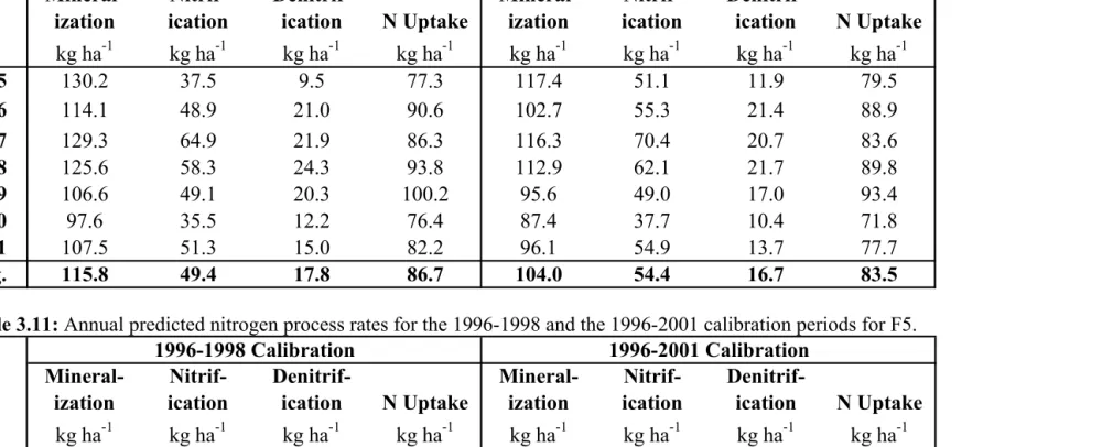
Table 3.10 Annual nitrogen process rates for the 1996-1998 and the 91 1996-2001 calibration periods for F3.
Table 3.11 Annual nitrogen process rates for the 1996-1998 and the 91 1996-2001 calibration periods for F5.
Table 3.12 Annual nitrogen process rates for the 1996-1998 and the 92 1996-2001 calibration periods for F6.
Table 3.13 Annual net mineralization rates from the literature. 92
APPENDIX A:
LIST OF FIGURES
CHAPTER 1:
Figure 1.1 Nitrogen cycle as modeled in DRAINMOD-N II 15 Figure 1.2 Carbon cycle as modeled in DRAINMOD-N II 15 CHAPTER 2:
Figure 2.1 Location of research site 56 Figure 2.2 Map of study area designating fields F3, F5, and F6 and indicators 56
for hydrology and water quality sampling locations.
Figure 2.3 Drainage versus height above weir to determine hydraulic 57 conductivity of F3 using flow data from 1996 and 1997.
Figure 2.4 Drainage versus height above weir to determine hydraulic 57 conductivity of F5 using flow data from 1996 and 1997.
Figure 2.5 Drainage versus height above weir to determine hydraulic 58 conductivity of F6 using flow data from 1996 and 1997.
Figure 2.6 Measured soil water characteristic for three layers in F3. 58 Figure 2.7 Measured soil water characteristic for three layers in F5. 59 Figure 2.8 Measured soil water characteristic for three layers in F6. 59 Figure 2.9 Estimates of drainable porosity from measured water table depth 60 responses to precipitation events in 1996-1997 and
1999-2000 for F3.
Figure 2.10 Estimates of drainable porosity from measured water table depth 60 responses to precipitation events in 1996-1997 and 1999 for F5.
Figure 2.11 Estimates of drainable porosity from measured water table depth 61 responses to precipitation events in 1996-1997 for F6.
Figure 2.12 Calibrated volume drained – water table depth relationships for 61 F3, F5, and F6.
Figure 2.13 Structure of the PnET-CN model with C/N representing pools 62 of carbon and nitrogen storage.
Figure 2.14 Monthly PnET-CN predicted drainage versus measured 62
drainage for F3.
Figure 2.15 Cumulative monthly PnET-CN predicted drainage versus 63 measured drainage for F3.
Figure 2.16 Normalized loblolly pine needlefall. 63 Figure 2.17 Monthly litterfall predictions for F3, F5, and F6. 64 CHAPTER 3:
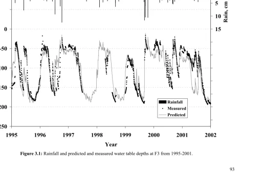
Figure 3.1 Rainfall and predicted and measured water table depths at F3 93
from 1995-2001.
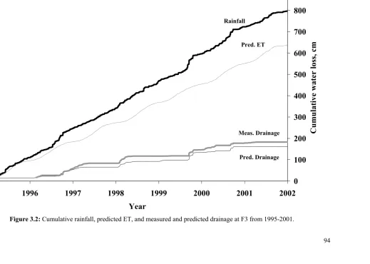
Figure 3.2 Cumulative rainfall, predicted ET, and measured and predicted 94 drainage at F3 from 1995-2001.
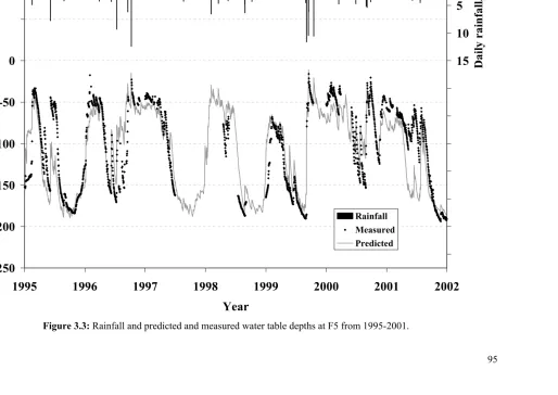
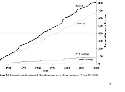
Figure 3.3 Rainfall and predicted and measured water table depths at F5 95
from 1995-2001.
drainage at F5 from 1995-2001.
Figure 3.5 Rainfall and predicted and measured water table depths at F6 97
from 1995-2001.
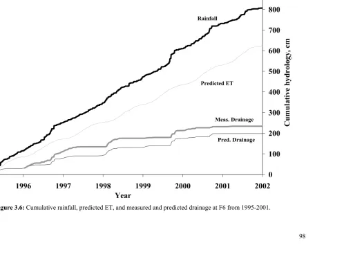
Figure 3.6 Cumulative rainfall, predicted ET, and measured and predicted 98 drainage at F6 from 1995-2001.
Figure 3.7 Rainfall and predicted and measured water table depths at F3 99
from 1995.
Figure 3.8 Predicted versus measured water table depths at F3 from 1995. 99 Figure 3.9 Rainfall and predicted and measured water table depths at F3 100
from 1996-1997.
Figure 3.10 Cumulative rainfall, predicted ET, and measured and predicted 100 drainage at F3 from 1996-1997.
Figure 3.11 Predicted versus measured water table depths at F3 from 101 1996-1997.
Figure 3.12 Predicted versus measured drainage rates at F3 from 1996-1997. 101 Figure 3.13 Rainfall and predicted and measured water table depths at F3 102
from 1998-1999.
Figure 3.14 Cumulative rainfall, predicted ET, and measured and predicted 102 drainage at F3 from 1998-1999.
Figure 3.15 Predicted versus measured water table depths at F3 from 103 1998-1999.
Figure 3.16 Predicted versus measured drainage rates at F3 from 1998-1999. 103 Figure 3.17 Rainfall and predicted and measured water table depths at F3 104
from 2000-2001.
Figure 3.18 Cumulative rainfall, predicted ET, and measured and predicted 104 drainage at F3 from 2000-2001.
Figure 3.19 Predicted versus measured water table depths at F3 from 105 2000-2001.
Figure 3.20 Predicted versus measured drainage rates at F3 from 2000-2001. 105 Figure 3.21 Rainfall and predicted and measured water table depths at F5 106
from 1995.
Figure 3.22 Predicted versus measured water table depths at F5 from 1995. 106 Figure 3.23 Rainfall and predicted and measured water table depths at F5 107
from 1996-1997.
Figure 3.24 Cumulative rainfall, predicted ET, and measured and predicted 107 drainage at F5 from 1996-1997.
Figure 3.25 Predicted versus measured water table depths at F5 from 108 1996-1997.
Figure 3.26 Predicted versus measured drainage rates at F5 from 1996-1997. 108 Figure 3.27 Rainfall and predicted and measured water table depths at F5 109
from 1998-1999.
Figure 3.28 Cumulative rainfall, predicted ET, and measured and predicted 109 drainage at F5 from 1998-1999.
Figure 3.29 Predicted versus measured water table depths at F5 from 110 1998-1999.
Figure 3.31 Rainfall and predicted and measured water table depths at F5 111
from 2000-2001.
Figure 3.32 Cumulative rainfall, predicted ET, and measured and predicted 111 drainage at F5 from 2000-2001.
Figure 3.33 Predicted versus measured water table depths at F5 from 112 2000-2001.
Figure 3.34 Predicted versus measured drainage rates at F5 from 2000-2001. 112 Figure 3.35 Rainfall and predicted and measured water table depths at F6 113
from 1995.
Figure 3.36 Predicted versus measured water table depths at F6 from 1995. 113 Figure 3.37 Rainfall and predicted and measured water table depths at F6 114
from 1996-1997.
Figure 3.38 Cumulative rainfall, predicted ET, and measured and predicted 114 drainage at F6 from 1996-1997.
Figure 3.39 Predicted versus measured water table depths at F6 from 115 1996-1997.
Figure 3.40 Predicted versus measured drainage rates at F6 from 1996-1997. 115 Figure 3.41 Rainfall and predicted and measured water table depths at F6 116
from 1998-1999.
Figure 3.42 Cumulative rainfall, predicted ET, and measured and predicted 116 drainage at F6 from 1998-1999.
Figure 3.43 Predicted versus measured water table depths at F6 from 117 1998-1999.
Figure 3.44 Predicted versus measured drainage rates at F6 from 1998-1999. 117 Figure 3.45 Rainfall and predicted and measured water table depths at F6 118
from 2000-2001.
Figure 3.46 Cumulative rainfall, predicted ET, and measured and predicted 118 drainage at F6 from 2000-2001.
Figure 3.47 Predicted versus measured water table depths at F6 from 119 2000-2001.
Figure 3.48 Predicted versus measured drainage rates at F6 from 2000-2001. 119 Figure 3.49 Measured and predicted cumulative drainage and nitrate loads 120
for F3 using 1996-1998 calibration.
Figure 3.50 Measured and predicted cumulative drainage and nitrate loads 120 for F3 using 1996-2001 calibration.
Figure 3.51 Measured and predicted nitrate concentrations for F3 using 121 1996-1998 calibration.
Figure 3.52 Measured and predicted nitrate concentrations for F3 using 121 1996-2001 calibration.
Figure 3.53 Measured and predicted cumulative drainage and nitrate loads 122 for F5 using 1996-1998 calibration.
Figure 3.54 Measured and predicted cumulative drainage and nitrate loads 122 for F5 using 1996-2001 calibration.
Figure 3.56 Measured and predicted nitrate concentrations for F5 using 123 1996-2001 calibration.
Figure 3.57 Measured and predicted cumulative drainage and nitrate loads 124 for F6 using 1996-2001 calibration.
Figure 3.58 Measured and predicted nitrate concentrations for F6 using 124 1996-2001 calibration.
APPENDIX A:
CHAPTER 1: INTRODUCTION
BACKGROUND
Nitrogen (N) loads from nonpoint source pollution have led to detrimental impacts on receiving waters in coastal regions (U.S. EPA, 1993). Nitrate-nitrogen (NO3-N) losses from
agricultural fields have been shown to increase N concentrations in groundwater and surface water, which can lead to contamination of drinking water supplies and eutrophication of receiving waters (Gilliam et al., 1999). While decreased water quality has been observed in response to artificial drainage on agricultural fields, uncertainty remains about the effect of drained forested fields on downstream water quality (Amatya et al., 1998).
Past work in eastern North Carolina has shown that nutrient exports from managed pine plantations can be similar to baseline exports from natural stands (Amatya et al., 1998). However, Chescheir et al. (2003) found that nutrient exports from managed pine plantations in eastern North Carolina vary significantly. The authors studied the effect of soil variability, vegetation, drainage intensity, and physiographic location on hydrology and nutrient export. They reported that variations in soil organic content can affect the nutrient export from forest sites. However, the impacts of vegetation, drainage intensity, and physiographic location were not evident in the database they studied. Vegetation can affect the amount of evapotranspiration (ET) at the site and therefore the drainage volume. Artificial drainage could increase total N losses because of an increase in drainage volume. In addition, poorly drained soils often have increased anaerobic zones where denitrification can occur, which could lower the concentration of NO3-N in outflow.
When forest management practices such as harvesting and fertilization are used, studies have shown that an increase in N export is possible, if only for a few months or years after the management event (Shepard, 1994). Several studies performed in the southeastern U.S. on drained forests have shown that harvesting can lead to increased N losses (Lebo et al., 1998; Fisher, 1981; Ensign et al., 2001). Harvesting alters the hydrology of the forest, and less N is removed through plant uptake. Nitrogen fertilization increases the amount of N in the system and can lead to increased N losses from forested fields.
Nitrogen transport in managed forests is a complex process. Soil variability,
method of simulating the combined effects of these factors to develop a better understanding of N transport in forests. Nitrogen models can also provide a useful method for developing and evaluating management practices for reducing N loads from forests.
DRAINMOD-N II –MODEL DESCRIPTION
DRAINMOD-N II was developed to simulate nitrogen dynamics and turnover in the
soil-water-plant system under different management techniques and soil conditions (Youssef, 2003). Driving hydrologic input parameters are determined from the water table
management model DRAINMOD 5.1 (Skaggs, 1978; Skaggs et al. 1991). The model simulates N transport using the multi-phase form of the one-dimensional,
advective-dispersive-reactive (ADR) equation. The model includes a detailed N cycle and a simplified carbon (C) cycle to simulate N dynamics and turnover in the soil-water-plant system under different management scenarios and soil conditions. DRAINMOD-N II model output includes daily predictions of NO3-N and ammonium-nitrogen (NH4-N) in the soil solution
and drainage outflow and cumulative rates of simulated N transformation processes.
DRAINMOD-N II has several improvements over the previous model, DRAINMOD-N
(Breve, 1994). These changes were necessary for simulating N fate and transport on highly organic forested fields. DRAINMOD-N uses a simplified N cycle, which did not consider NH4-N as a mineral pool. Chescheir et al. (2003) found that losses of NH4-N from forested
fields in eastern North Carolina can be significant. DRAINMOD-N also did not consider amending soils with organic N sources or temporal changes in soil organic nitrogen (ON) content. Litterfall from trees in forests adds a significant amount of organic N to the soil every year; therefore, the old version of the model could not simulate forest N cycling accurately. Since the old version of the model did not consider temporal changes in ON content, it would be impossible to accurately simulate N cycling for several consecutive years. The new version of the model considers NH4-N as a mineral pool, ON amendment,
and temporal changes in ON content. The model also has an improved denitrification
Nitrogen Cycle
DRAINMOD-N II considers a detailed N cycle that includes three N pools: NO3-N,
ammoniacal nitrogen (NHX-N), and organic nitrogen (ON) (Youssef, 2003). The NHX-N
pool, which includes ammonia-nitrogen (NH3-N) and NH4-N, can be ignored for
simplification if it is reasonable to do so based on environmental and soil conditions. As shown in Figure 1.1, the model considers the following N transformation processes: atmospheric deposition, application of mineral N fertilizers, application of ON sources, N plant uptake, N mineralization and immobilization, nitrification, denitrification, NH3
volatilization, and NO3-N and NHX-N losses due to leaching and surface runoff (Youssef,
2003).
Carbon Cycle
The availability of C is an important factor to consider when modeling N dynamics, especially in highly organic forested systems. Denitrification requires available C to proceed, and the processes of mineralization and immobilization are a consequence of C cycling in the soil-water system. DRAINMOD-N II simulates C dynamics and turnover based on a simplified C cycle (Youssef, 2003). As shown in Figure 1.2, it includes three soil organic matter (SOM) pools: active, slow, and passive as well as two added organic matter (AOM) pools: metabolic and structural. The SOM pools refer to organic carbon (OC) that is present in the soil as opposed to AOM, which refers to OC that is added through application of manures or crop residues. Each pool of organic matter is characterized by its OC content, potential rate of decomposition, and its carbon-to-nitrogen (C:N) ratio. In addition, each pool has a corresponding ON pool, and the five pools comprise the one ON pool shown in Figure 1.1. The active pool has the fastest turnover rate among the SOM pools, followed by the slow pool and then the passive pool. The active pool includes microbial biomass and metabolites, the slow pool represents more stable decomposition products, and the passive pool represents the most stable OM.
Modes of Operation
DRAINMOD-N II has three different modes of operation. The first mode, ‘basic
environmental conditions permit. The second mode, ‘normal mode’, considers NO3-N and
NH4-N, and the third mode, ‘volatilization mode’, considers NO3-N, NH3-N, and NH4-N. If
the NHX-N pool is considered, the model automatically switches between normal and
volatilization modes according to soil pH.
Governing Equation
DRAINMOD-N II uses a multi-phase form of the one-dimensional
advection-dispersion-reaction (ADR) equation to simulate N transport. The equation is ‘multi-phase’ because it considers the gaseous, aqueous, and solid phases of N species transport. It is ‘one-dimensional’ because the N transport is described in the vertical direction from the soil surface to the top of the impermeable layer. Transport through advection is mass transfer in the aqueous phase that occurs due to a hydraulic gradient. Transport through dispersion occurs due to molecular diffusion and mechanical dispersion (Wong, 2003). Nitrogen species can be accumulated or depleted based on several microbial processes, and the equation describes this with a source/sink term.
The multi-phase form of the one-dimensional ADR equation, written in terms of species in the aqueous phase, is the following,
S z C z C H d D z C K H t a a a g g a a a d b g
a ∂ +
∂ − ∂ ∂ + ∂ ∂ = + + ∂ ∂ θ θ ρ θ θ (ν ) (1.1)
where θaandθgare the volumetric fractions [L3L-3] of the aqueous and gaseous phases,
respectively, ρbis the dry bulk density of the solid phase [ML-3], Kd is the distribution
coefficient [L3M-1], H is Henry’s coefficient, Cais the species concentration [ML-3] in the
aqueous phase, Da is the coefficient of hydrodynamic dispersion [L2T-1] that characterizes
dispersive transport in the aqueous phase, dgis the molecular diffusion coefficient [L2T-1]
that characterizes diffusive transport in the gaseous phase, νais the volumetric flux of the
aqueous phase [LT-1], S is a source/sink term [ML-3T-1] that characterizes additional
processes (plant uptake, transformations, etc.), t is time [T], and z is a spatial coordinate [L] (Youssef, 2003).
The source/sink term describes the cumulative affect of a number of N transformation processes on a particular N species. The source/sink term for NHX-N can be defined as
S = Shyd+ Smin,NH4+ Sdep,NH4+ Sfer,NH4 – Simm,NH4– Snit – Supt,NH4 – Srnf,NH4 (1.2)
where Shydis urea hydrolysis rate, Smin,NH4 is ammonium mineralization rate, Sdep,NH4 is rate of
ammonium deposition through precipitation, Sfer,NH4 is ammonium fertilization rate, Simm,NH4
is ammonium immobilization rate, Snit is rate of ammonium lost by nitrification, Supt,NH4 is
rate of ammonium plant uptake, and Srnf,NH4 is the rate of ammonium lost in surface runoff
(all units in [ML-3T-1]).
The source/sink term for NO3-N is defined by,
S = Sdep,NO3 + Sfer,NO3 + Snit+ Smin,NO3 – Simm,NO3 – Sden – Supt,NO3 – Srnf,NO3 (1.3)
where Sdep,NO3is rate of nitrate deposition through precipitation, Sfer,NO3is nitrate fertilization
rate, Smin,NO3is nitrate mineralization rate, Simm,NO3is nitrate immobilization rate, Sdenis the
denitrification rate, Supt,NO3is rate of nitrate plant uptake, and Srnf,NO3is rate ofnitrate lost in
surface runoff (all units in [ML-3T-1]). Nitrate mineralization occurs only if the model is run in basic mode, which does not consider NHX-N. Nitrate immobilization will occur only if
the NHx-N pool is depleted.
Carbon and Nitrogen Transformations
Effect of Environmental Factors on C and N Transformations
Most processes affecting C and N transformations in the soil-water system are driven by microbial activity. Any changes in the soil-water environment that affect microbial activity will have an impact on C and N transformation rates. Youssef (2003) described the effect of soil temperature, soil moisture, and soil pH on C and N transformations by defining a dimensionless response function for each factor. An overall response function that
describes the cumulative effect of these environmental factors is defined using a linear combination the individual response functions. The C and N transformation process rates are defined in the model as follows,
k = fe kopt (1.4)
where k is the actual process rate, koptis the optimum process rate, assuming ideal
environmental conditions, and fe is the dimensionless overall response factor that takes values
from 0 to 1.
In DRAINMOD-N II, the effect of pH on microbial processes is set to be optional.
fe= ft fsw (1.5)
where ftis the temperature response function and fsw is the soil water response function. If
the effect of pH is included, the two most influential factors are used to quantify fe,
fe = min{ft fsw, ft fpH, fsw fpH} (1.6)
where fpH is the pH response function.
The temperature response function, ft, is based on a form of the Van’t Hoff equation
with variable Q10,
)] / 5 . 0 1 ( 5 . 0
exp[ opt opt
t T T T T
f = − β +β − (1.7)
where βis an empirical coefficient, T is temperature [oC], Topt is the optimum temperature
[oC] at which ft equals unity. As temperature increases, microbial activity increases to a
threshold value. If the temperature continues to increase, microbial activity begins to decline.
In DRAINMOD-N II, two soil water response functions were developed. One
function was developed for denitrification, which proceeds optimally at complete saturation and decreases to zero as the water content decreases to a certain threshold saturation. The other function was developed for the other C and N transformation processes, which have a range of saturation values below complete saturation in which the process proceeds
optimally. If the soil water content exceeds or is less than the optimum saturation range, the process rate will be limited (Youssef, 2003).
The soil water response function for denitrification, fsw,dn, is defined as,
≥ − − < = dn e dn dn dn dn
sw s s
s s s
s s
f , 1
1 0
(1.8)
where s is the relative saturation, dimensionless, sdnis a threshold relative saturation,
dimensionless, below which denitrification does not occur, and e1 is an empirical exponent (Youssef, 2003).
≤ ≤ − − − + ≤ ≤ ≤ < − − − + = l wp e wp l wp wp wp u l u e u s s sw s s s s s s s f f s s s s s s s f f f 2 2 ) 1 ( 1 1 1 1 ) 1 ( (1.9)
where suand sldefine the upper and lower limits of the relative saturation range within which
the biological proceeds at optimum rate, swpis the relative saturation at permanent wilting
point, fsand fwpare the values of the soil water function at saturation, and permanent wilting
point, respectively, and e2 is an empirical exponent (Youssef, 2003). The pH response function is defined as,
≤ < − − − + ≤ ≤ < ≤ − − − + = max 3 max max max max min 3 min min min min ) 1 ( 1 ) 1 ( pH pH pH pH pH pH pH f f pH pH pH pH pH pH pH pH pH pH f f f u e u u l l e l
pH (1.10)
where pHmin and pHmaxare the limits of the pH range that could occur in the system, pH1 and
pHudefine the upper and lower bounds of a pH range within which the transformation
proceeds at the optimum rate, fminand fmaxare the values of the response function at pHminand
pHmax, respectively, and e3 is an empirical exponent (Youssef, 2003).
Application of Animal Waste and Crop Residues
DRAINMOD-N II was originally developed for agricultural systems and simulates the
lignin-to-nitrogen (L:N) ratio, and its OC content. Organic matter that is added is divided into the metabolic and structural pools, based on its lignin-to-nitrogen (L:N) ratio,
Fmet= 0.85 – 0.018LNRadd (1.11)
Fstr = 1 - Fmet
where Fmetand Fstrare the metabolic and structural fractions of added OM, respectively, and
LNRadd is the lignin-to-nitrogen ratio of added OM. This method separates the slowly
decomposable fraction of OM, which is represented by the lignin content, from the readily decomposable fraction.
When OM is added to the structural and metabolic pools, the OC content of both pools changes. The C:N ratio of the metabolic pool changes depending on the C:N ratio of the added OM. The structural pool OC decomposition rate is a function of the lignin content and a potential decomposition rate. Therefore, when OM is added the structural pool
decomposition rate changes (Youssef, 2003).
Organic C Decomposition and N Mineralization/Immobilization
N mineralization and immobilization is a result of carbon cycling between pools (Youssef, 2003). The total amount of OC released from a given pool j, OCrel,j [MM-1T-1], is
given by,
OCrel,j = fe Kdec,j OCj (1.12)
where fe is a dimensionless environmental response function, Kdec,j is a first order
decomposition rate constant [T-1], and OC
j is the OC content of pool j [MM-1]. As OC is
released from the various pools, some OC is potentially available for N mineralization to occur.
The gross N mineralization that occurs due to the OC release from a given pool j, Nmin,j [MM-1T-1], is given by,
j j rel j
CNR OC
Nmin, = , (1.13)
where CNRj is the C:N ratio of pool j.
OCsyn,jk = αjk ejkOCrel,j (1.14)
where αjk is a dimensionless mass fraction of OC released from pool j and resynthesized into
pool k and ejkis a dimensionless synthesis efficiency factor for OC flow from pool j into pool
k.
The gross N immobilization that occurs due to OC moving from one pool to other available pools, Nimm,j [MM-1T-1], is determined by,
∑
= k k jk syn j imm CNR OCN , , (1.15)
The net N mineralization or immobilization associated with C flows for all pools is given by,
∑
− = j j imm j a bimm N N
Smin/ ( min, , )
θ ρ
(1.16)
where Smin,imm is the rate of net N mineralization/immobilization [ML-3T-1].
Nitrification
In DRAINMOD-N II, nitrification is modeled using Michaelis-Menten kinetics with
respect to NH4-N and is described by,
+ = a b NH nit m NH nit inh e nit C K C V f f S θ ρ 4 , 4 max, (1.17)
where fe is the dimensionless environmental response function, finhis a dimensionless
response function for nitrification inhibitors, Vmax,nitis the maximum nitrification rate
[MM-1T-1], Km,nit is the half-saturation constant [MM-3], the substrate concentration at which
the reaction rate is half Vmax,nit,and CNH4 is the ammonium concentration [MM-1] (Youssef,
2003).
The nitrification process is limited if the ammonium concentration is below a threshold value and the process behaves as a first-order function. Once the ammonium concentration reaches a threshold value, nitrification rate is no longer limited by ammonium supply and the process proceeds as a zero-order function. DRAINMOD-N II simulates the effect of any added nitrification inhibitors on nitrification rate by using the response function,
finh, which has values from 0 to 1 based on the concentration of nitrification inhibitors in the
Denitrification
In DRAINMOD-N II, denitrification rate is represented using Michaelis-Menten
kinetics with respect to NO3-N,
+ = a b NO NO m NO den z e den C K C V f f S θ ρ 3 3 , 3 max, (1.18)
where Sdenis the denitrification rate [ML-3T-1], Vmax,denis the maximum denitrification rate
[MM-1T-1], CNO3 is the NO3-N concentration [ML-3], and Km,NO3is the NO3-N half-saturation
constant [ML-3]. Organic C availability has been shown to be important in regulating denitrification rates. The influence of OC is simulated using a empirical function relating carbon availability with depth,
fz= e-αz (1.19)
where α is an empirical exponent, and z is the depth from the soil surface [L] (Youssef, 2003).
Plant Uptake
Plant uptake for NO3-N and NH4-N is simulated in DRAINMOD-N II by using the
following functions, + = 3 4 3 3 3 , min NO NH NO NO upt NO upt N N N N S
S (1.20)
+ = 4 4 3 4 4 , min NH NH NO NH upt NH upt N N N N S S (1.21)
where Supt,NO3and Supt,NH4 are the actual uptake rates [ML-3T-1] from the NO3-N and NH4-N
pools, respectively, and NNO3 and NNH4 are the sum of the aqueous and solid phase
concentrations [ML-3] of NO
3-N and NH4-N, respectively.
root upt crp
upt D
f N
S = (1.22)
where Ncrp is the total amount of N taken up by plants during the growing season
[ML-2], fupt is the fractional N-uptake demand [T-1], which is given as an empirical N-uptake
versus growing season relationship, and Droot [L] is the effective rooting depth.
The model assumes that NO3-N and NH4-N are both equally available to plants, and
the plants take the N species up in relative proportions. When one N species is used up, the plant will take up N from the remaining species pool. When N demand exceeds available N, the plant takes up whatever N is left and N stress occurs. The model does not simulate the effect of N stress on crop yield.
Atmospheric Deposition
Functions for atmospheric deposition to the surface layer are defined as follows,
z fC
S rainNO
NO
dep = ∆
3 ,
3 (1.23)
z fC
S rainNH
NH
dep = ∆
4 , 4
, (1.24)
where Sdep is the rainfall deposition rate [ML-3T-1], Crain,NO3 and Crain,NH4are the NO3-N and
NH4-N concentrations in rain, respectively, and f is the infiltration rate.
Surface Runoff
Surface runoff loss of aqueous N species is quantified using the following equation,
z C q
Srnf X rnf rnf X
∆
= ,
, (1.25)
where Srnf,X is the rate of NO3-N or NH4-N loss in runoff [ML-3T-1], qnrfis runoff rate [LT-1]
as predicted by DRAINMOD and Crnf,Xis the concentration [ML-3] of NO3-N or NH4-N in
MODEL TESTING
Field testing of the DRAINMOD 5.1/DRAINMOD-N II models was conducted using six years (1992-1997) of data from an experimental site in the Lower Coastal Plain of North Carolina, near Plymouth (Youssef et al, 2003a; Youssef et al, 2003b). The model was tested for a corn-wheat-soybean rotation on four 1.7-ha fields under conventional (free) and
controlled drainage. The authors stressed that the test of the model should be regarded as incomplete, since most input parameters were not measured in the field or laboratory. Automatic measurements were taken of water table depth midway between drains,
subsurface drainage flow rates, and meteorological data. Flow-proportional NO3-N samples
were taken from subsurface drainage biweekly or more frequently during high-flow events. The hydrologic simulation model DRAINMOD 5.1 was shown to produce ‘good’ results when comparing predicted and measured values of water table depth. The predicted water table depth was between 11.8-13.9 cm of measured values on average for the four fields. The average coefficient of determination (R2) for water table depth was between 0.71 and 0.77, showing good agreement.
Predictions of subsurface drainage rates showed ‘generally good’ agreement between observed drainage rates. The absolute normalized error was 5.7 and 12.1 % between
observed and predicted drainage rates. The average R2 values were 0.65 to 0.73 for the four fields, which shows ‘fair to good’ agreement. The authors cited the underprediction of drainage rates during high flow events as the primary cause of disagreement (Youssef et al., 2003a).
DRAINMOD-N II was used to predict annual NO3-N leaching losses and the results
were compared with measured values. The average absolute normalized error for annual NO3-N losses in subsurface drainage were 19.9 – 46.0 %, which showed ‘fair to good’
agreement. However, the absolute normalized error in predicting NO3-N leaching losses was
less than 25 % in half of the 24 simulated fieldxyears. The authors stated that errors in predicting water table depth and drainage rates were the primary causes of disagreement and noted a strong influence of the hydrologic predictions of DRAINMOD 5.1 on the
DRAINMOD-N II did an ‘excellent’ job in predicting cumulative NO3-N leaching
losses over the entire six-year simulation period. Cumulative NO3-N leaching losses were
overpredicted by 2.1 % for one plot and underpredicted by 5.9-10.2 % for the other three plots. Although there were sometimes large discrepancies between observed and predicted annual NO3-N leaching losses, prediction errors in cumulative NO3-N losses were very small
(Youssef et al., 2003b).
The authors stated that the results of the field modeling showed the potential for the widespread use of DRAINMOD-N II to simulate N dynamics and turnover in agricultural ecosystems. They stressed that further research should be conducted to test the model with independent measurements of model input parameters before widespread use (Youssef et al., 2003b).
MODELING FORESTED CONDITIONS
DRAINMOD-N II was originally developed and tested for application in agricultural
systems. Since it incorporates a detailed N cycle as well as a simplified C cycle,
DRAINMOD-N II should be able to simulate N transport and turnover in forested systems
with accurate parameterization and a few minor modifications.
DRAINMOD-N II estimates potential plant uptake of NO3-N and NH4-N as a function
of relative yield, which is predicted by DRAINMOD 5.1. Relative yield in DRAINMOD 5.1 is predicted for each growing season as a function of different growth stresses on the crop. A new relative yield is predicted for each crop and for each growing season. However, trees grow continually from year to year, and the current plant uptake method inadequately
describes the cumulative effect of each year’s climate on forest development. Therefore, it is necessary to develop an estimate of potential N uptake for a given year that depends on the physiological development of the forest.
DRAINMOD-N II simulates the application of organic material such as manure and
climate factors, such as heavy rainfall and winds. It is necessary to develop a method to estimate foliar production and to simulate variable application of litterfall.
In a comprehensive study of nutrient export from forests in eastern North Carolina, Chescheir et al. (2003) found that annual total nitrogen exports were typically less than 7.5 kg ha-1 yr-1. However, the authors reported that annual N losses from some fields with highly organic soils in that study were significantly higher, with loads as high as 23.9 kg ha-1 yr-1. These highly organic soils have hydrologic characteristics, such as very high saturated conductivities in the top layers, which are not well understood. In addition, there is
uncertainty in the rates of certain N transformation processes, which could explain the higher N losses. A study of these forested fields would be useful for DRAINMOD-N II model evaluation and for developing a better understanding of the field properties that affect the hydrology and N losses from these fields.
OBJECTIVES
The goal of this study is to accurately model nitrogen loading at the field scale for three forests in the Coastal Plain of eastern North Carolina using DRAINMOD-N II. Specific objectives of the project are:
1. To accurately model the hydrology of three forested fields using DRAINMOD. 2. To determine litterfall and N uptake at the study sites and develop methods in
DRAINMOD-N II to quantify these processes.
Figure 1.1 Nitrogen cycle as modeled in DRAINMOD-N II (Youssef, 2003)
REFERENCES
Amatya, D. M., J. W. Gilliam, R. W. Skaggs, M. E. Lebo, and R. G. Campbell. 1998. Effects of controlled drainage on forest water quality. J. Environ. Qual. 27:923-935.
Brevé, M. A. 1994. Modeling the movement and fate of nitrogen in artificially drained soils. Unpublished Ph.D. dissertation, North Carolina State University, Raleigh, N. C. Chescheir, G. M., M. E. Lebo, D. M. Amatya, J. Hughes, J. W. Gilliam, R. W. Skaggs,
and R.B. Herrmann. 2003. Hydrology and Water Quality of Forested Lands in Eastern North Carolina. Technical Bulletin 320. Raleigh, N.C.: North Carolina State University.
Ensign, S. H., and M. A. Mallin. 2001. Stream water quality changes following timber harvest in a coastal plain swamp forest. Wat. Res. 35(14):3381-3390.
Fisher, R. F. 1981. Impact of intensive silviculture on soil and water quality in a coastal lowland. In Tropical Agricultural Hydrology: Watershed Management and Land Use. R. Lal and E. W. Russell, eds. New York, NY.: John Wiley & Sons Ltd.
Gilliam, J. W., J. L. Baker, and K. R. Reddy. 1999. Water quality effects of Drainage in Humid regions. In Agricultural Drainage, 801-830. R. W. Skaggs and J. van Schilfgaarde, eds. Madison, WI. Agron. Monogr. 38. ASA, CSSA, and SSSA. Lebo, M. E., and R. B. Herrmann. 1998. Harvest impacts on forest outflow in coastal North
Carolina. J. Environ. Qual. 27:1382-1395.
Shepard , J. P. 1994. Effects of forest management on surface water quality in wetland forests. Wetlands. 14(1):18-26.
Skaggs, R. W. 1978. A water table management model for shallow water table soils. Rept. 134. Raleigh, N.C.: North Carolina Water Resources Res. Inst., North Carolina State University.
Skaggs, R. W., T. Karvonen, and H. Kandil. 1991. Predicting soil water fluxes in drained lands. ASAE Meeting Paper No. 91-2090. St. Joseph, MI.: ASAE.
U.S. Environmental Protection Agency. 1993. Guidance specifying management measures for sources of nonpoint pollution in coastal waters.EPA-840-B-92-002. Washington, D.C.: Office of Water, U.S. EPA.
Wong, T. 2003. Mechanisms of Solute Transport. Stony Brook, NY.: Stony Brook
University. Available at: wellspring.ess.sunysb.edu/~wong/geo515/outline924.pdf. Accessed 7 November 2003.
Youssef, M. A., R. W. Skaggs, G. M. Chescheir, and J. W. Gilliam. 2003a. Field evaluation
of DRAINMOD 5.1 using six years of data from an artificially drained agricultural
field in North Carolina. ASAE Meeting Paper No. 032367. St. Joseph, MI.: ASAE. Youssef, M. A., R. W. Skaggs, G. M. Chescheir, and J. W. Gilliam. 2003b. Field testing of
DRAINMOD-N II for North Carolina soils. ASAE Meeting Paper No. 032368. St.
CHAPTER 2: METHODS
SITE DESCRIPTION
To test the accuracy of DRAINMOD-N II on forested fields, seven years (1995-2001) of hydrologic and water quality data were recorded from three managed loblolly pine forests in the Lower Coastal Plain of North Carolina. The three forested fields are located in
Weyerhaeuser’s Parker Tract near the town of Plymouth and are designated as F3, F5, and F6, as shown in Figures 2.1 and 2.2.
Field – F3
Field F3 is 47 ha and was planted with loblolly pine in 1983. The field is nearly flat and has open ditches for water table management that are spaced approximately 80-m apart and 1.0-m deep with an outlet weir maintained at an elevation 0.70 m below the average soil surface. The soil is classified as the Cape Fear series (fine, mixed, semiactive Typic
Umbraquult). As observed in the field, the soil is dark sandy loam in the top 25 cm with 5-15 % organic matter, sandy clay loam at 25 to 60 cm depth, sandy loam at 60 to 75 cm depth, and gray sandy clay from 75 to 155 cm depth.
Field – F5
Field F5 is 128 ha and was planted with loblolly pine in 1984 and partially thinned in late September 2000. The nearly flat field has open ditches that are approximately 100-m apart and 1.0-m deep with an outlet weir maintained at an elevation 0.70 m below the average soil surface. The soil is classified as the organic Belhaven (Loamy, mixed, dysic, thermic Terric Haplosaprists) and Pungo (Dysic, thermic Typic Haplosaprists) series. As observed in the field, the soil is a black to reddish brown, mucky organic (25-90 % OM) in the top 45 cm, dark yellowish brown loam at 45 to 70 cm depth, and brown sandy loam at 70 to 150 cm depth.
Field – F6
series. As observed in the field, the soil is a very dark brown to black organic (20-95 % OM) in the top 50 cm and dark greyish brown sandy loam at 50 to 85 cm depth. Observations were not made below 85 cm depth, but it is reasonable to assume properties similar to F5 below that depth.
HYDROLOGY MEASUREMENTS
Weather
Rainfall was collected from 1995-2001 using automatic recorders at two locations (R1 and R6) as shown in Figure 2.2. Automatic tipping bucket gauges were used and the number of tips was recorded using an electronic datalogger (Onset Hobo ® or Omnidata ® event loggers). The data were downloaded every two weeks, and manual gauges were used to back up and provide calibration for the automatic measurements.
R6 was also the site of a full weather station, which measured air temperature, wind speed, relative humidity, net radiation, solar radiation, and rainfall. Data were recorded every 30 minutes using a Campbell Scientific CR10X datalogger ®.
Water Table
Water table depth measurements were made in the center of each field at the midpoint between two drainage ditches (Figure 2.2) from 1995-2001. Water table monitoring wells were constructed out of 4-in. PVC pipe and screened at various depths. Water table
elevations were recorded using a float-and-pulley system and an automatic datalogger (Blue Earth Research ST485 ® or Omnidata ®). The float and pulley system was replaced with an Infinity 222 ® datalogger in 2001. Data from the dataloggers were downloaded about every two weeks and any necessary calibrations were made at that time.
Flow
®). The upstream stage was also measured using a chart recorder for verification and backup of the digital system. The data were downloaded every two weeks and any necessary
calibrations were made at that time.
With a V-notched weir and upstream and downstream stage measurements, it is possible to calculate the drainage outflow rate from a given field, even during submergence. When the downstream water level was below the weir invert, the following equation was used to determine the flow rate over a sharpcrested, 120o V-notched weir (Grant and Dawson, 2001),
Q = 4.33 H 2.5 (2.1)
where Q is the flow rate (ft3 s-1) and H is the upstream water stage above the V notch (m). When the weir was submerged, the following equation was used to determine the flow rate (Brater et al., 1996),
(
)
0.5 0.3852 1 5
. 2 1 * 1
36 . 4 − = H H H
Q (2.2)
where H1is the upstream height of water above the bottom of the V notch (ft), and H2is the
downstream height of water above the bottom of the V notch (ft). Very infrequently, data from both the digital automatic recorders and the charts would be unavailable. In such cases, estimates of stage were made using data from other nearby fields, which were instrumented for other studies. Resulting measurements, in this case, were treated as approximate.
WATER QUALITY MEASUREMENTS
kept on ice until they could be put in a laboratory freezer, where they remained frozen until analysis. Concentrations of NO3-N and NH4-N were measured colormetrically with a Lachat
Quickchem 8000 Instrument, using standard methods (APHA, 1992).
Samplers were in flow-proportional, composite mode most of the time. When the samplers were in discrete mode, sufficient samples were taken so that linear interpolation could be used to estimate daily nutrient concentrations between measurements. The daily nutrient export load was determined by multiplying the nutrient concentration by the measured outflow volume for each day.
HYDROLOGY SIMULATIONS
Modeling Scenario
Hydrology simulations were performed with the water table management model
DRAINMOD 5.1 (Skaggs, 1978; Skaggs et al., 1991). Calibration of the model input
parameters was performed using measured water table elevation and drainage data from 1996-2001. The extensive calibration period was required due to the difficulty in
determining accurate input parameters for the highly organic and highly porous soils and because of relatively long periods of missing water table elevation data. The accuracy of
DRAINMOD-N II predictions is very dependent on the accuracy of the DRAINMOD
hydrology predictions (Youssef, 2003). Therefore, it was important to have the most accurate hydrology simulations possible to accurately assess DRAINMOD-N II model predictions. Hydrologic simulations of 1995 were also performed for each field to establish the initial condition for the DRAINMOD-N II simulations.
DRAINMOD Model Description
DRAINMOD was developed to characterize drainage and water table control practices
in flat (<2.0 % slope), poorly drained soils. The model is based on a water balance for a section of soil midway between two parallel drains, which may be either open ditches or buried drain tubes. The model can be applied for open ditches by simulating very large subsurface drains. The section of soil has a unit surface area and extends from the
∆Va= D + ET + DS – F (2.3)
where ∆Va is the change in air volume or water free pore space (cm), D is the drainage (cm)
from the section, ET is evapotranspiration (cm), DS is deep seepage (cm), and F is infiltration (cm).
A separate water balance is used to determine the volume of infiltration, runoff, and surface storage that occurs in response to precipitation,
P = F + ∆S + RO (2.4)
where P is precipitation (cm), ∆S is the change in volume of water in surface storage (cm), and RO is runoff (cm).
The water balance is calculated in 1-h increments on days with rainfall. If no rainfall occurs, the time step is two hours. If rainfall does not occur and drainage is low, the time step is one day. If the rainfall rate exceeds the infiltration capacity, time increments of
≤ 0.1 h are used for infiltration calculations.
Infiltration
The Green-Ampt equation describes infiltration and is given by,
f = Ks + Ks Md Sf F (2.5)
where f is the infiltration rate (cm/h), F is the cumulative infiltration (cm), Ksis the vertical
hydraulic conductivity of the transmission zone (cm/h), Mdis the difference between final
and initial volumetric water contents (cm3 cm-3), and Sfis the effective suction at the wetting
front (cm). DRAINMOD uses a simplification of the Green-Ampt equation for a given soil with a given initial water content,
f = A / F + B (2.6)
where A (cm2 h-1) and B (cm h-1) are parameters that depend on soil properties, initial water content and distribution, and surface conditions. The infiltration parameter A is defined as,
A = Ks Md Sf (2.7)
Surface Drainage
There are two parameters that describe surface drainage in DRAINMOD. The maximum surface storage (cm) defines the amount of water that can be stored on the soil surface before surface runoff begins. Kirkham’s depth for flow to drains (cm) represents the storage in small depressions due to surface cover characteristics and surface grading.
Kirkham’s depth is used when predicting subsurface drainage during ponded conditions.
Subsurface Drainage
The model uses the Hooghoudt equation (Bouwer and van Schilfgaarde, 1963) to predict subsurface drainage based on water table elevation by assuming an elliptical water table profile between drains and assuming horizontal streamlines in the saturated region. The Hooghoudt equation is a steady state function, but it can be applied using small time steps because the water table drawdown is typically very slow (Bouwer and van Schilfgaarde, 1963). The Hooghoudt equation is given by,
2 2 8 4
L Kmd Km
q= + e (2.8)
where q is the drainage flux, (cm h-1), m is the midpoint water table height above the drain (cm), K is the effective lateral hydraulic conductivity (cm h-1), L is the drain spacing (cm), and deis the equivalent depth of the impermeable layer below the drain (cm). Equations to
solve for the equivalent depth were determined by Moody (1967) and are computed internally in DRAINMOD.
When water is ponded above Kirkham’s depth, water on the surface can move freely and most of the flow will be concentrated near the ditches. In this situation, the assumption of horizontal streamlines does not hold and another method is required. The model uses Kirkham’s equation (Kirkham, 1957) to predict outflow when the water on the surface is ponded above Kirkham’s depth.
Evapotranspiration
appropriate method from atmospheric data. PET is a function of net solar radiation,
temperature, humidity, and wind velocity. Different methods are chosen based primarily on atmospheric data availability. PET represents the maximum amount of water that will be removed from the soil system by evaporation and transpiration when sufficient soil water is available.
Once PET is determined, a check is made to determine if soil water conditions are limiting. The soil water content at the lower limit is defined as the water content below which plants can no longer obtain water. If the soil water content is greater than the lower limit, ET is equal to PET. If the soil water content is less than the lower limit, ET is limited to the rate that upward flux supplies water to the root zone. The upward flux is the transfer of water in the unsaturated zone through capillary action from the vicinity of the water table to the root zone. If sufficient water is available through upward flux, ET is equal to PET. If sufficient water is not available through upward flux, ET demand is satisfied by removing water from the root zone, creating a dry zone. When the dry zone encompasses the root zone, ET is limited to the upward flux rate.
DRAINMOD Input Parameters
Weather
Measured hourly precipitation data from the R1 gauge were used for the F3
simulation, and data from the R6 gauge were used for the F5 and F6 simulations. Monthly average rainfall for the duration of the study is shown in Table 2.1. Since a full weather station was available at R6, the Penman-Monteith method was used to estimate PET from 1996-2001 for each simulation (Monteith, 1965).
Drainage System Parameters
Drainage system parameters include inputs that describe surface and subsurface components of the drainage system. The maximum surface storage is the volume of water that must be filled before surface drainage can occur. In a forested system, surface drainage is typically very poor; the maximum surface storage (STMAX) was set to be 10 cm for F3 and 15 cm for F5 and F6. Kirkham’s depth (STORRO) was set to be 5 cm for F3 and 10 cm for F5 and F6.
Subsurface drainage parameters include inputs that describe drain depth and spacing, drain effective radius, drain hydraulic capacity (drainage coefficient), depth to impermeable layer, and height of controlled drainage structures. The drain effective radius was set to be 30 cm for all fields, which is used to describe open ditches. It was assumed that the ditches would provide enough drainage capacity for the peak drainage rates. The drainage
coefficients were set to values higher than the highest measured drainage rate for each field. The depth to impermeable layer was not measured in the field, but it was estimated to be 250 cm for all fields, which is just below the lowest measured water table depth for the six years of measurements.
Saturated Hydraulic Conductivity
Since artificial drainage primarily involves lateral flow to drains, a very important input parameter in DRAINMOD is lateral saturated hydraulic conductivity. Hydraulic conductivity describes the resistance to water flow through the soil. Hydraulic conductivity in F3 was measured using the auger hole method (van Beers, 1970), and the results are shown in Table 2.3. However, the auger hole method only provides an estimate of saturated conductivityat a single point in the field, and it only represents a limited depth of the soil profile. In fields F5 and F6, the lateral saturated hydraulic conductivities are too high to measure using this method. Therefore, it was necessary to calibrate this parameter for input
to DRAINMOD.
Hooghoudt equation, 4 2 2
L Km
, describes the flow that occurs above the drain, or in the case of
ditches, the flow that occurs above the water surface in the ditch. The second term, 8 2
L m Kde
,
describes the flow that occurs below the water level in the ditch. It is possible to separate the hydraulic conductivity for the entire profile, K, into an effective conductivity, Ke,for the soil
above the ditch bottom and another conductivity, Kb, for the soil below the ditch bottom.
The effective conductivity of the soil above the drain, Ke, can then be separated into as many
layers as necessary as shown by,
n i i n n i i i i e L L L L K L K L K K + + + + + + = + + + ... ... 1 1
1 (2.9)
where Ki is the saturated lateral hydraulic conductivity of layer i, and n is the number of
layers, and Li is the depth of layer i. If the Hooghoudt equation is combined with equation
2.9, a relationship between water table depth and drainage outflow can be formed. The new relationship is a function of the drainage system properties and the individual conductivities of a multi-layered soil system as shown by,
2 1 1 1 2 8 ... ... 4 L md K L L L L K L K L K m q e b n i i n n i i i i + + + + + + + = + + + (2.10)
A plot of measured height above the weir, m, versus measured drainage outflow, q,
was constructed for each field for two years of data (1996-1997). To determine the flow rate for a given elevation, the height of the water table was taken in consideration. For example, if the water table reached the middle of the top layer, the depth of the top layer, Li, would be
equal to one-half Li. If the water table reached the bottom of the top later, Liwould be equal
to zero, and so on. In this way, the proper weight would be given to each layer in determining the flow rate for different water table depths.