ABSTRACT
MOKASHI, ANUP CHANDRAKANT. The Simulation Start-up Problem: Performance Comparison of N-Skart and MSER-5. (Under the direction of James R. Wilson.)
The objective of this research is to conduct an extensive performance comparison of the batch-means
procedures MSER-5 and N-Skart in terms of their effectiveness in handling the simulation start-up
prob-lem. Given a fixed-length simulation-generated time series that is potentially contaminated by a tran-sient effect arising from the simulation’s initial condition, the deletion approach for the treatment of the
simulation start-up problem is to determine a data-truncation point (or warm-up period) beyond which
the observations have approximately steady-state behavior and thus can be used to compute point and confidence-interval (CI) estimators of the steady-state mean. MSER-5 uses the data-truncation point
that minimizes the half-length of the usual batch-means CI based on batches whose size is always 5
ob-servations. N-Skart applies a randomness test to spaced batch means in order to determine sufficiently large sizes for each batch and its preceding spacer such that beyond the initial spacer (which is taken to
define the data-truncation point), the spaced batch means are approximately independent of each other
and the simulation’s initial condition; then using truncated nonspaced batch means, N-Skart exploits separate adjustments to the CI half-length that account for the effects on the distribution of the
underly-ing Student’s t-statistic arisunderly-ing from skewness and autocorrelation of the batch means. To compare both the methods in terms of the accuracy and reliability of their point and CI estimators of the steady-state
mean, the experimental performance comparison used fixed-length simulation output sequences
exhibit-ing patterns of initialization bias that are representative of many real-world simulation output processes. The results provide substantial evidence that the point estimator delivered by N-Skart generally has
sub-stantially smaller bias, variance, and mean-squared error than that delivered by MSER-5; moreover in
© Copyright 2010 by Anup Chandrakant Mokashi
The Simulation Start-up Problem: Performance Comparison of N-Skart and MSER-5
by
Anup Chandrakant Mokashi
A thesis submitted to the Graduate Faculty of North Carolina State University
in partial fulfillment of the requirements for the Degree of
Master of Science
Industrial Engineering
Raleigh, North Carolina
2010
APPROVED BY:
Peter Bloomfield Russell E. King
DEDICATION
BIOGRAPHY
Anup Chandrakant Mokashi was born on October 14, 1986, in the city of Satara, India. He was raised
by his parents, Mr. Chandrakant Y. Mokashi and Mrs. Shubhada C. Mokashi, along with his brother
Archit.
In the fall of 2004, he entered the Bachelor of Engineering Program in the Pune University system.
He graduated with a degree in mechanical engineering in 2008. In the fall of 2008, he began his graduate
study in industrial engineering at North Carolina State University. He has also worked as a teaching assistant in the Edward P. Fitts Department of Industrial and Systems Engineering at North Carolina
ACKNOWLEDGEMENTS
I would like to express my sincere gratitude to Dr. James R. Wilson for introducing me to the field of
stochastic simulation and for the time and effort that he has spent in helping me with my research. It
was a privilege for me to work under his guidance. I would like to thank Dr. Ali Tafazzoli Yazdi for his help and contributions during my research. I would like to thank Dr. Russell E. King for serving
on my advisory committee and for his help as the Director of Graduate Programs on various occasions
TABLE OF CONTENTS
List of Tables . . . vi
List of Figures . . . vii
Chapter 1 Introduction . . . 1
1.1 Problem Statement and Research Objectives . . . 1
1.2 Organization of the Thesis . . . 2
Chapter 2 Literature Review . . . 4
2.1 The Simulation Start-up Problem . . . 4
2.2 Review of Previous Literature on the Simulation Start-up Problem . . . 6
2.3 Overview of N-Skart and MSER5 . . . 14
2.3.1 MSER5 . . . 14
2.3.2 N-Skart . . . 16
Chapter 3 Performance Comparison of N-Skart and MSER-5 . . . 20
3.1 Measures for Comparison of N-Skart and MSER-5 . . . 20
3.2 Description of Test Problems . . . 22
3.2.1 M/M/1 Queue-Waiting-Time Process with Empty Initial Condition and 90% Utilization . . . 22
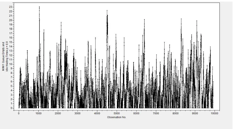
3.2.2 M/M/1 Queue-Waiting-Time Process with Empty Initial Condition and 80% Utilization . . . 30
3.2.3 M/M/1 Queue-Waiting-Time Process with 113 Initial Customers and 90% Uti-lization . . . 37
3.2.4 First-Order Autoregressive (AR(1)) Process . . . 45
3.2.5 AR(1)-to-Pareto (ARTOP) Process . . . 53
Chapter 4 Conclusions and Future Research . . . 62
4.1 Conclusions . . . 62
4.2 Contributions of the Current Research . . . 64
4.3 Directions for Future Research . . . 64
References . . . 66
LIST OF TABLES
Table 3.1 Performance of MSER-5 and N-Skart in the M/M/1 queue-waiting-time
pro-cess with 90% server utilization and empty-and-idle initial condition . . . 24
Table 3.2 Performance of MSER-5 and N-Skart in the M/M/1 queue-waiting-time
pro-cess with 80% server utilization and empty-and-idle initial condition . . . 31
Table 3.3 Performance of MSER-5 and N-Skart in the M/M/1 queue-waiting-time
pro-cess with 90% server utilization and 113 initial customers . . . 39
Table 3.4 Performance of MSER-5 and N-Skart in the AR(1) process . . . 47
LIST OF FIGURES
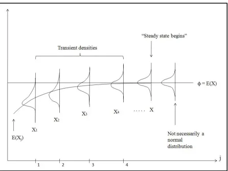
Figure 2.1 Transient and steady-state density functions for a particular stochastic process
X1,X2, . . .and initial conditionX0 . . . 5
Figure 2.2 Flowchart of MSER-5 . . . 16
Figure 2.3 Flowchart of N-Skart . . . 19
Figure 3.1 A realization of theM/M/1 queue-waiting-time process with empty-and-idle
initial condition and 90% server utilization . . . 23
Figure 3.2 Empirical distributions of truncated sample mean for N-Skart, MSER-5, and
modified MSER-5 when applied to M/M/1 queue-waiting-time process with
X1=0,ρ=0.9, andN=10,000 . . . 25
Figure 3.3 Empirical distributions of truncated sample mean for N-Skart, MSER-5, and
modified MSER-5 when applied to M/M/1 queue-waiting-time process with
X1=0,ρ=0.9, andN=20,000 . . . 26
Figure 3.4 Empirical distributions of truncated sample mean for N-Skart, MSER-5, and
modified MSER-5 when applied to M/M/1 queue-waiting-time process with
X1=0,ρ=0.9, andN=50,000 . . . 27
Figure 3.5 Empirical distributions of truncated sample mean for N-Skart, MSER-5, and
modified MSER-5 when applied to M/M/1 queue-waiting-time process with
X1=0,ρ=0.9, andN=200,000 . . . 28
Figure 3.6 A realization of theM/M/1 queue-waiting-time process with empty-and-idle
initial condition and 80% server utilization . . . 30
Figure 3.7 Empirical distributions of truncated sample mean for N-Skart, MSER-5, and
modified MSER-5 when applied to M/M/1 queue-waiting-time process with
X1=0,ρ=0.8, andN=10,000 . . . 32
Figure 3.8 Empirical distributions of truncated sample mean for N-Skart, MSER-5, and
modified MSER-5 when applied to M/M/1 queue-waiting-time process with
X1=0,ρ=0.8, andN=20,000 . . . 33
Figure 3.9 Empirical distributions of truncated sample mean for N-Skart, MSER-5, and
modified MSER-5 when applied to M/M/1 queue-waiting-time process with
X1=0,ρ=0.8, andN=50,000 . . . 34
Figure 3.10 Empirical distributions of truncated sample mean for N-Skart, MSER-5, and
modified MSER-5 when applied to M/M/1 queue-waiting-time process with
X1=0,ρ=0.8, andN=200,000 . . . 35
Figure 3.11 A realization of theM/M/1 queue-waiting time process with 113 initial
cus-tomers and 90% server utilization . . . 37
Figure 3.12 A depiction of the transient behavior of theM/M/1 queue-waiting time process
with 113 initial customers and 90% server utilization for 3 independent replications 38
Figure 3.13 Empirical distributions of truncated sample mean for N-Skart, MSER-5, and
modified MSER-5 when applied to M/M/1 queue-waiting-time process with
Figure 3.14 Empirical distributions of truncated sample mean for N-Skart, MSER-5, and
modified MSER-5 when applied to M/M/1 queue-waiting-time process with
113 initial customers,ρ=0.9, andN=20,000 . . . 41
Figure 3.15 Empirical distributions of truncated sample mean for N-Skart, MSER-5, and
modified MSER-5 when applied to M/M/1 queue-waiting-time process with
113 initial customers,ρ=0.9, andN=50,000 . . . 42
Figure 3.16 Empirical distributions of truncated sample mean for N-Skart, MSER-5, and
modified MSER-5 when applied to M/M/1 queue-waiting-time process with
113 initial customers,ρ=0.9, andN=200,000 . . . 43
Figure 3.17 A realization of the AR(1) Process (3.7)X0=0,µX =100, andρ=0.995 . . 45
Figure 3.18 A depiction of the transient behavior of the AR(1) Process (3.7)X0=0,µX =
100, andρ=0.995 for 3 independent replications . . . 46
Figure 3.19 Empirical distributions of truncated sample mean for N-Skart, MSER-5, and
modified MSER-5 when applied to AR(1) process (3.7) withX0=0,µX=100,
ρ=0.995, andN=10,000 . . . 48
Figure 3.20 Empirical distributions of truncated sample mean for N-Skart, MSER-5, and
modified MSER-5 when applied to AR(1) process (3.7) withX0=0,µX=100,
ρ=0.995, andN=20,000 . . . 49
Figure 3.21 Empirical distributions of truncated sample mean for N-Skart, MSER-5, and
modified MSER-5 when applied to AR(1) process (3.7) withX0=0,µX=100,
ρ=0.995, andN=50,000 . . . 50
Figure 3.22 Empirical distributions of truncated sample mean for N-Skart, MSER-5, and
modified MSER-5 when applied to AR(1) process (3.7) withX0=0,µX=100,
ρ=0.995, andN=200,000 . . . 51
Figure 3.23 A realization of the ARTOP Process . . . 54
Figure 3.24 A depiction of the transient behavior of the ARTOP Process for 3 independent
replications . . . 55
Figure 3.25 Empirical distributions of truncated sample mean for N-Skart, MSER-5, and
modified MSER-5 when applied to ARTOP process (3.12) withN=10,000 . . 57
Figure 3.26 Empirical distributions of truncated sample mean for N-Skart, MSER-5, and
modified MSER-5 when applied to ARTOP process (3.12) withN=20,000 . . 58
Figure 3.27 Empirical distributions of truncated sample mean for N-Skart, MSER-5, and
modified MSER-5 when applied to ARTOP process (3.12) withN=50,000 . . 59
Figure 3.28 Empirical distributions of truncated sample mean for N-Skart, MSER-5, and
modified MSER-5 when applied to ARTOP process (3.12) withN=200,000 . 60
Figure 1 C Code for N-Skart . . . 69
Chapter 1
Introduction
Simulation studies have become an important tool in the modeling and analysis of real-world systems.
Typically, we are interested in knowing about the characteristics of a dynamic stochastic system in its long-run steady-state operational condition. Steady-state (nonterminating) simulation, unlike a
termi-nating simulation, does not have any specified starting or stopping conditions. As a result, the
parame-ters of interest that are to be estimated are defined over time as the time horizon tends to infinity. While designing nonterminating simulation experiments, an arbitrary starting condition is chosen and the
sim-ulation is run for a sufficient number of output responses so as to approximate the long-run average
behavior of the system. Ideally, the starting condition should not affect the estimates of the parameters of interest. However, the starting condition introduces a transient in the simulation output responses
which results in biased estimates of the steady-state parameters of interest. The problem of initialization
bias has been a long-standing problem in the field of simulation modeling and analysis and has been the subject of several studies conducted in the past.
1.1. Problem Statement and Research Objectives
In this study, the problem of initialization bias is described in detail, and an overview is provided of the
various approaches used for the treatment of initialization bias in simulation output processes. Special
emphasis is given to the truncation approach, and a detailed explanation is presented for the intuition behind this approach. Various methods employing the truncation rationale are described, and two of
the methods proposed in recent times are selected for comparison—namely, N-Skart (Tafazzoli, Steiger,
and Wilson 2010) and MSER-5 (Franklin and White 2008).
N-Skart (Tafazzoli, Steiger, and Wilson 2010) is a nonsequential procedure designed to deliver
a confidence interval (CI) for the steady-state mean of a simulation output process when a single simulation-generated time series of arbitrary size is supplied by the user, and a required coverage
determine sufficiently large sizes for each batch and its preceding spacer such that beyond the initial
spacer (which is taken to define the data-truncation point), the spaced batch means are approximately
independent of each other and the simulation’s initial condition; then using truncated, nonspaced batch means, N-Skart makes separate adjustments to the half-length of the CI in order to account for the effect
of skewness and autocorrelation of the batch means on the underlying Student’st-statistic. If the sample
size is large enough, N-Skart delivers a point estimate and a CI for the steady-state mean of the process that is approximately free of initialization bias.
MSER-5 (Franklin and White 2008) is a variant of the MSER procedure first proposed by White
(1997). It is a truncation heuristic for resolving the start-up problem which has received a consider-able amount of attention in recent times due to its simplicity. Given a finite sequence, MSER-5 first
computes batch means from adjacent (nonoverlapping) batches, each consisting of five observations;
then MSER-5 computes the usual CI for the steady-state mean based on the assumption that the batch means are randomly sampled from a normal distribution; and finally MSER-5 sequentially recomputes
the batch means CI after deleting (truncating) progressively more initial batch means until the width of the marginal confidence interval about the truncated sample mean is minimized. The truncated sequence
can then be considered to be approximately free of initialization bias; and the corresponding truncated
sample average of the batch-means is supposed to have minimal mean-squared error as an estimator of the steady-state mean. Moreover, the usual batch means CI for the steady-state mean computed from
the batch means beyond MSER-5’s “optimal” truncation point is supposed to be a valid CI—that is, its
actual coverage probability should be (nearly) equal to the user-specified nominal coverage probability. MSER-5 and N-Skart are compared in terms of their effectiveness in removing the initial transient
for a carefully selected set of test problems with patterns of initialization bias that are typical of many
large-scale simulation applications. Four different sample sizes are used to test the effectiveness of the methods for large, medium, and relatively small output streams. The performance of the two methods
is analyzed both in terms of the following:
(a) Statistics that are indicative of the residual initialization bias after truncation; and
(b) Graphs of those statistics.
Consistency of the performance of both the methods is tested by performing 1,000 independent
replica-tions for both N-Skart and MSER-5 on 1,000 independent realizareplica-tions of each test process.
1.2. Organization of the Thesis
The remainder of the thesis is organized as follows: Chapter 2 presents a brief overview of the
performance for the comparison of the two methods along with the experimental design of the test
prob-lems selected for the comparison. Chapter 4 presents the results of the experiments. Chapter 5 contains
Chapter 2
Literature Review
2.1. The Simulation Start-up Problem
Simulation studies are primarily conducted in order to obtain reliable information about parameters of interest, which cannot be readily obtained through analytical methods. For the analysis of
simula-tion output, we use several statistical methods. Most of these statistical methods are applied under the
assumptions that the simulation output observations are independent and identically distributed. How-ever, many real world processes and simulations are nonstationary and correlated. Consider a stochastic
output process from a single simulation run given byX1,X2,X3, . . .. In general, the process can be
ex-pressed as{Xj}for j=1,2,3, . . .. These successive observations in this process, in general, will neither
be independent nor identically distributed; moreover in many simulation-generated responses are not
even approximately distributed according to a normal distribution. As a result, conventional
statisti-cal methods (such as the usual confidence interval based on Student’st-distribution) cannot be applied
directly.
For above defined simulation output process, let the initial condition at the start of the simulation be represented by X0. Let Fj(x|X0) =P(Xj ≤x|X0), where Fj(x|X0) is the transient distribution of
the process at time j, for initial condition X0. The transient distribution varies for different values
of j and X0. If Fj(x|X0)→F(x) as j→∞ for all x and for any initial conditions X0, then F(x) is called the steady-state distribution of the output processX1,X2,X3. . .. Ideally,Fj(x|X0)→F(x) only
as j→∞; but in practice, there will be a finite time index beyond which these distributions would be
approximately the same as each other. Thus, ifdis such a point which satisfies this condition, then each
observationXjwith index j>dcan be said to have been sampled approximately from the steady-state
distribution. Also, the individual observations{Xj: j=d+1,d+2, . . .}would not be independent, but
are assumed to constitute an approximately covariance stationary process. The steady-state distribution
F(x)is independent of the initial condition X0, but the rate of convergence ofFj(x|X0)toF(x)is not.
convergence of the transient probability distributions of the random variable{Xj} to the steady-state
distribution as j→∞.
Figure 2.1: Transient and steady-state density functions for a particular stochastic processX1,X2, . . .
and initial conditionX0
The simulation for a particular system may be terminating or nonterminating depending on the
objectives of the study. A terminating simulation is one for which a specified eventE determines the
length of each simulation run. A nonterminating simulation does not have any such event to determine
the end of a replication. The measures of performance of a terminating or nonterminating simulation are
greatly influenced by the state of the system at the beginning of the simulation run, represented byX0.
Suppose we are interested in determining a steady-state parameterφ; i.e. a parameter of the steady-state
distributionF(x)of a nonterminating simulation. One practical difficulty in estimatingφ is that we are
trying to estimate the parameters of a distributionF(x)which would be obtained only as j→∞, but in
steady-state parameter of interest. Also, it is not always possible to choose the initial conditionX0that
is representative of the steady-state behavior of the system. Thus, if we are trying to estimate
φ=E(X) =
Z +∞
−∞
xdF(x), (2.1)
i.e., the steady state mean of the process, then the sample mean
Xn=
1
n n
∑
i=1
Xi (2.2)
will be a biased estimator of φ for all values of n. This problem is called as the initialization-bias
problem or the simulation start-up problem.
2.2. Review of Previous Literature on the Simulation Start-up Problem
Conway (1963) discussed the artificiality introduced in a simulation output due to its abrupt starting,
unlike the real world system it represents, and the resulting deviation from equilibrium conditions in
steady-state operation. He elaborated the effect of initial conditions on the stochastic dependence be-tween observations in both steady-state and transient simulations. He also suggested truncation as an
efficient method of removing the effect of initial conditions and proposed a rule for truncation wherein
the initial set of observations were deleted until the first of the residual series was neither the maximum nor the minimum. Another approach suggested by him was to start the simulation using initial
condi-tions that are representative of the steady state. This would help to shorten, if not eliminate, the time required for a simulation to reach equilibrium conditions.
Fishman (1972) investigated the effect of the initial transient in a simulation output on the
steady-state mean of a process, using the first-order autoregressive process as a test problem. Fishman proposed that the bias in the simulation output is directly proportional to the deviation of the initial condition from
the steady-state parameter of interest and inversely proportional to the run length of the simulation. He
also investigated the effect of truncating an initial set of observations on the bias and variance of the simulation output. In the results presented, he questioned the effectiveness of the truncation method
against the resulting increase in variance in the truncated output sequence.
Welch (1983) defined the start-up problem as follows: with respect to a particular estimand, the problem is to identify a truncation point beyond which the expected value of the estimate of the
pa-rameter of interest is approximately equal to its limiting value. He proposed a graphical solution to
the start-up problem which requires the user to perform multiple replications of the system. The mean and the variance at any point in simulated time can be estimated by averaging the corresponding
val-ues across all replications. On theith independent replication of the simulation, fori=1, . . . ,k,letXi j
initial condition for each replication. An estimate of the transient mean function
µj(X0) =E[Xi j|X0] =
Z +∞
−∞
xdFj(x|X0) for j=1, . . . ,n, (2.3)
is the sample average transient mean function
b
µj(X0) = 1
k k
∑
i=1
Xi j for j=1, . . . ,n, (2.4)
which is the sample mean response computed at the time index j, averaged across all k replications.
Similarly, an estimate of the transient variance function
σ2j(X0) =Var[Xi j|X0] =
Z +∞
−∞
{x−E[Xi j|X0]}2dFj(x) for j=1, . . . ,n (2.5)
is the sample variance
b
σ2j(X0) = 1
k−1
k
∑
i=1
[Xi j−bµj(X0)] 2
for j=1, . . . ,n, (2.6)
of all the responses observed at timej, computed across allkreplications. Thus, an approximate 100(1−
α)% confidence interval forµj(X0)is
b
µj(X0)±t1−α/2,k−1 b σj(X0)
√
k , (2.7)
wheret1−α/2,k−1is the(1−α)quantile of Student’st-distribution withk−1 degrees of freedom. Welch
proposed identifying the enddof the warm-up period (that is, the truncation point) by visual inspection
of the sample average transient mean function (2.4) or of the confidence band (2.7) so that for the time
index j≥d, (2.4) or (2.7) have “settled down” and thus, approximately represent steady-state behavior.
In this case, the truncated sample mean on replicationi
Xi(n,d) =
1
n−d n
∑
j=d+1
Xi j for i=1, . . . ,k, (2.8)
is an approximately unbiased estimator of the steady-state meanµX=
Z +∞
−∞
xdF(x); and a 100(1−α)%
confidence interval forµX is
X(k,n,d)±t1−α 2,k−1
SX(n,d)
√
k , (2.9)
where
X(k,n,d) =1 k
k
∑
i=1
and
S2X(n,d)= 1 k−1
k
∑
i=1
[Xi(n,d)−X(k,n,d)]
2
(2.11)
are the grand mean and the sample variance of the truncated sample means, respectively. To smooth out the short-term fluctuations in the sequence, Welch recommended the use of moving averages which
would reduce the sensitivity of the simulation output data to these irregularities.
Gafarian, Ancker, and Morisaku (1977) proposed that a random variable was to be used to estimate the true truncation point. They suggested the following criteria for evaluating performance of various
truncation rules:
• Accuracy — The ratio of expected value of the truncation point to the true truncation point should
be close to 1;
• Precision — The coefficient of variation of the estimate of the truncation point should be close to
0;
• Generality — The truncation rule should perform well for a broad range of systems;
• Simplicity — The rule should be easy to implement for average practitioners; and
• Cost — Expenses in computer time required should be minimum.
Wilson and Pritsker (1978a, 1978b) presented a survey of the various start-up policies in practice
which define the initial conditions and the truncation point in a simulation output process. They classi-fied the policies into three broad categories as follows.
• time series models;
• queueing models; and
• heuristic rules of thumb.
They provided an overview of the various statistics used to evaluate start-up policies and stressed the importance of developing appropriate performance measures in order to compare the alternative start-up
policies in a consistent manner. The suggestion put forward by them with respect to truncation rules
was to develop an evaluation procedure for all the truncation methods that would focus on the behavior of the truncated sample mean and would consider the random variation in the truncation point. The
evaluation procedure should also be able to characterize the random and systematic components of the
The resulting evaluation procedure developed by them used the bias, variance and mean-squared
error of the truncated sample mean along with the confidence interval coverage for performance
com-parison of start-up policies which were defined as a combination of initial condition rules (ICi) and
truncation rules(T Rl). Given a simulation output process denoted by{Xj : j=1, . . . ,n}, the various
initial condition rules and truncation rules used in their evaluation procedure are as follows.
Initial Condition rules:
• IC1 →Start the system “empty and idle”.
• IC2 →Set the initial conditionX0as close to the steady-state mode as possible.
• IC3 →Set the initial conditionX0as close to the steady-state mean as possible.
Truncation rules:
• T R0 →Retain all data.
• T R1 →Set the truncation pointdsuch that the observationXd+1in the given sequence is neither
maximum nor minimum of the remaining sequence{Xj: j=d+1, . . . ,n}.
• T R2 →Set the truncation point asd=nwhen the simulation output sequence{Xj}has crossed
its meanXnat leastk−1 times i.e.{sgn(Xt−Xn) : 1≤t≤n}containskruns.
• T R3 →Setd=nwhen the batch-means ofkmost recent batches of sizebfall within an interval
of lengthε.
The steps in the evaluation procedure can be summarized as follows.
1. Compute the bias, variance and mean-squared error for all the start-up policies of interest(ICi,T Rl).
2. Estimate the distribution of the truncation pointd over independent simulation runs for each of
the start-up policies.
3. Calculate the averaged values of the bias, variance and mean-squared-error.
4. Select a base policy. Calculate the half-length of a nominal 100(1−α%)confidence interval (CI)
for the steady state meanφ based on individual replications. Obtain the standard average
half-length of the CI for the base policy. Adjust the nominal confidence level for all other policies so
that the half-length of the resulting confidence intervals is the same as for the policy.
5. Compute coverage probabilities for all possible values of the truncation point d for individual
replications of each start-up policy. Averaged CI coveragesCn(i,l)are calculated for each
On applying the above comprehensive evaluation procedure to a single-server queue (M/M/1/15
queue with arrival rateλ =4.5 and service rateµ =5) and a machine repair system (M/M/3/14/14
queue with failure rate λ =0.2 and repair rate µ =0.5), it was observed that specifying an initial
condition close to the steady-state mode was optimal. This is because departure from this condition
resulted in increased variance and reduced CI coverage. Also, with respect to improving the estimate of
the steady-state mean, selection of initial condition played a more crucial role than truncation because the truncation rules under study were extremely sensitive to parameter misspecification which resulted
in considerable loss of CI coverage. It was also observed that incorporating prior information about the
process under study into the evaluation procedure significantly reduced the variability in the results. Law (1983) presented a comprehensive overview of the various statistical analysis techniques for
simulation output data. Specifically, for steady-state simulation analysis, he categorized the output
analysis techniques as fixed-sample-size procedures or sequential procedures. He further classified the fixed-sample-size procedures as:
• those that seek independent observations;
• those that seek to estimate dependence among output responses;
• those that exploit special structure of the underlying process; and
• those based on standardized time series.
Law (1983) also presented an in-depth analysis of the various techniques employed for mitigation of the start-up problem. He evaluated the deletion approach with respect to the following criteria:
• covariance stationarity;
• point-estimator quality; and
• confidence-interval quality.
A brief description of the same is presented below.
Output analysis techniques such as batch means, autoregressive representation, and spectrum
analy-sis, which are typically employed when we conduct a single long run of the simulation, assume that the
underlying process is covariance stationary. If our goal is to apply the above techniques to a covariance stationary process, then the truncation rationale used should ensure that the residual observations in the
truncated sequence are approximately covariance stationary.
Another approach for evaluating the efficiency of truncation is to consider the properties of the point estimator for some steady-state performance measure of interest such as the steady-state mean; and then
we are interested in the bias and variance of the truncated sample mean as an estimator of the
the steady-state mean for most processes but also cautioned regarding exceptions to this trend. When
considering the variance, if observations at the beginning of the output sequence have particularly large
variances, then truncation could decrease the variance of the estimator. Truncation also reduces the mean-squared error when the initialization bias is high and the observations are highly correlated. Also,
as the overall sample size increases, generally the ratio of the truncation point to the overall run length
(sample size) decreases.
The third approach for determining the efficiency of truncation is to assess its impact on the
confidence-interval quality. For a single long run of the simulation, the truncation approach does not have any
significant impact when the sample size is moderate and the methods employed for constructing the confidence interval are batch means, autoregressive representation, or spectrum analysis. If the number
of truncated observations is very large relative to the actual sample size, then truncation could actually
result in a degradation in the confidence-interval coverage. As against this, Law (1983) showed that replication and deletion, when used in conjunction, provided improved results. For a fixed sample size,
truncation increased the expected value of the confidence-interval half length. Also, truncation generally decreases the replication length required.
Kelton (1989) investigated the feasible methods for initializing simulations that would lead to lower
estimator bias or less requisite deletion. He compared deterministic and stochastic initialization rules and suggested forms for the initial distribution using the maximum entropy principle. His work can be
summarized as follows. The initialization states of steady-state simulations can be broadly classified as
deterministicorstochastic. Starting each simulation run in an identical deterministic state is the most
common method of initializing replications. Each replication, when initialized by the above method,
will pass through a transient phase that is identical across replications, since the initial state is always
the same; however, it must be recognized that on independent replications of the simulation model with the same starting state, the observed responses will exhibit different patterns of variation about the
transient mean function defined in equation (2.3). Therefore even when the same deterministic starting
date is used on each independent replication of the simulation, different realizations of the target output process that are conditionally independent of each other, given the simulation’s starting state.
Alternatively, one can draw the initial state from some probability distribution instead of
speci-fying it to be the same deterministic value for all replications. Thus, we can allow for different re-alized initialization states across replications and yet retain the probabilistic identity of the
replica-tions. In the absence of sufficient information regarding the form of the initial distribution, one can
utilize the principle of maximum entropy which produces a discrete probability mass function (p.m.f.) {p(x1),p(x2), . . . ,p(xk)} of a random variableX on the finite domain{x1, . . . ,xk}that maximizes the
p.m.f.’s entropy
H(p) =−E[ln(X)] =−
k
∑
i=1
subject to thetexpectation constraints
k
∑
i=1
gj(xi)p(xi) =νj for 1≤ j≤t. (2.13)
where
νj→specified constants
gi→given real-valued functions
Thus, we can express the problem as
max
p H(p) subject to
k
∑
i=1
p(xi) =1 and (2.13) (2.14)
The p.m.f. resulting from entropy maximization is the ”maximally noncommittal” distribution that
obeys the constraints. In the absence of any information regarding the expected system state in steady state, a discrete uniform distribution can be specified whose limits can be determined through a set of
initial pilot runs. Kelton used the following initialization methods for comparison:
• the batch means method for a single long run of the simulation;
• the replication method without deletion of the warm-up period;
• the replication method with deletion of the warm-up period;
• uniform initial distribution without deletion of the warm-up period;
• uniform initial distribution with deletion of the warm-up period;
• geometric initial distribution without deletion of the warm-up period; and
• geometric initial distribution without deletion of the warm-up period.
The evaluation criteria for the different methods were as follows.
• plots of the expected transient response as a function of discrete time;
• the percent bias; and
• the time required to attain near-steady state.
Kelton concluded that the stochastic initialization methods performed considerably better than the
repli-cation and batch-means methods with respect to reducing the bias in the simulation output and also
methods are considerably higher than the other methods. The primary drawback of stochastic
initial-ization is that in complex, large-scale simulations, it is exceedingly difficult if not impossible to do the
following:
(a) construct the relevant joint distribution of all the system state variables that define the simulation’s
initial state; and then
(b) randomly sample from the joint distribution in (a).
Starting the simulation in some convenient starting state and then clearing statistics at the end of a warm-up period of appropriate length—that is, using data truncation to solve the simulation start-up
problem—may be viewed as one method for stochastic initialization, because the system status at the
end of the warm-up period may be regarded as a probabilistically assigned initial condition for the simulation-generated output responses that are recorded beyond the end of the warm-up period.
Grassmann (2008) questioned the utility of the truncation approach for determining the steady state
of simulation output process. He proposed that if one starts a simulation with an initial state that has a high equilibrium probability, there should not be a warm-up period. He compared different starting
states for a number of systems and calculated the mean-squared error (MSE) for these different initial
states using the Markov modeling approach and the Markov event system (MES) as a modeling tool. Grassmann used the following test problems to illustrate his conclusions:
• a one-server queue;
• multiserver queues; and
• tandem queues.
He observed that starting the system in with different initial states did not affect the MSE
signifi-cantly. Specifically, for the one-server queue, selecting the starting value according to the equilibrium
probabilities yielded the largest MSE compared with a few other fixed starting states. He further noted that if the system under consideration regenerates (i.e. the same stochastic initial state is revisited), then
the utility of the truncation approach is questionable since the warm-up period at the beginning of each
regeneration cycle would be required to be truncated.
Grassmann also observed that in simulation outputs, the difference between variance and the MSE
becomes negligible as the sample size increases and the variance is strongly influenced by extreme
values . He questioned the utility of the MSE as a performance measure and suggested that it be replaced by an alternative measure such as the mean absolute deviation.
The main difficulty with Grassmann’s recommendation to use a fixed starting state with a relatively
large steady-state probability is related to the problem of implementing Kelton’s recommendation to use a randomly sampled starting state—in complex, large-scale simulations, both recommendations are
2.3. Overview of N-Skart and MSER5
2.3.1. MSER5
MSER-5 (Franklin and White 2008) is a modification of the Marginal Confidence Rule (MCR) or the
Marginal Standard Error Rule (MSER) proposed by White (1997). There are two key notions about the
intuition behind MSER-5:
• MSER-5 optimizes the objective function that we care the most about in simulation studies— i.e.,
the confidence interval (CI) for the steady-state meanµ; and
• MSER-5 provides a reasonable method for determining the approximate end of the warm-up
period.
MSER-5 aims at balancing improved accuracy achieved through reduction in the bias of the
esti-mate of the steady-state mean, with decreased precision due to reduction in sample size. It follows the rationale that given an output sequence{X1,X2, . . . ,XN}of length (sample size)N, the observations later
in the sequence provide a more accurate estimate of the central tendency at steady state; and hence, the initial observations, which are suspected to be further from the steady-state mean, should be truncated.
The heuristic works backwards in time gathering more and more observations. As long as these
obser-vations are representative of the steady state, the estimate of the width of the confidence interval around the estimate of the steady-state mean will continue to decrease. As soon as the observations collected
are not representative of the steady state behavior, the width of the confidence interval would start to
increase. Thus, the initial observations in the output sequence should be truncated to the extent that deleting those observations minimizes the length of the confidence interval for the steady-state mean
based on the remaining output sequence. The improvement of MSER-5 over MCR is that it batches
together 5 observations in the output sequence in order to ensure better behavior in the confidence inter-val. Therefore, MSER5 uses as its basic data items, the batch means computed from the original process {Xi:i=1, . . . ,N}with batch size 5,
Zj=
1 5
5j
∑
i=5(j−1)+1
Xi for j=1, . . . ,k=bN/5c. (2.15)
In terms of the batch means{Zj: j=1, . . . ,k}, MSER-5 determinesd∗, the optimal number of batches
in the warm-up period, as follows:
d∗=arg min
0≤d<k−1
z1−α/2SZ(k,d)
√
k−d , (2.16)
where:
z1−α/2denotes the(1−α/2)quantile of the standard normal distribution; and
Z(k,d) = 1 k−d
k
∑
j=d+1
Zj; (2.17)
andS2Z(k,d)denotes the corresponding truncated sample variance,
S2Z(k,d) = 1 k−d
k
∑
j=d+1
[Zj−Z(k,d)]
2
. (2.18)
The MSER-5 truncation criterion can then be expressed as
MSER5(k,d) = S 2
Z(k,d)
k−d ; (2.19)
and the truncation pointdis set to minimize MSER5(k,d)for 0≤d<k. The final point estimator of
the steady-state mean delivered by MSER-5 is the truncated sample meanZ(k,d∗); and the associated
nominal 100(1−α)% confidence interval forµ is
Z(k,d∗)±z1−α/2SZ(k,d ∗) √
k−d∗ . (2.20)
It has been observed that MSER-5 can sometimes deliver a truncation point at the end of the data
series—that is,d∗=k−2. According to Delaney (1995) and Spratt (1998), this is because the method
can be overly sensitive to observations at the end of the data series that are close in value. Spratt (1998)
proposed that this error can be avoided, partially, by not allowing the algorithm to consider the standard error calculated from the last few data points. Hence, while calculating the MSER-5 truncation criterion,
instead of using a minimum sample of 2 batches to calculate the truncated sample varianceS2Z(k,d), we
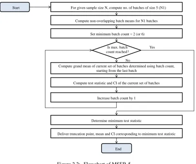
choose an arbitrarily greater sample size. Thus, we can summarize MSER-5 as a sequential procedure which utilizes a modified version of the nonoverlapping batch means procedure in order to deliver a
truncation point and a mean estimate with a 100(1−α)% CI for a simulation output sequence.
In Chapter 3, we evaluate the performance of MSER-5 in terms of the point and CI estimators ofµX
for a wide range of test processes. We consider the results obtained from the original N-Skart algorithm
as well as the results obtained from the modified algorithm with the correction proposed by Delaney
and Spratt. For the modified algorithm, we consider a minimum of 6 batches for calculating the sample varianceS2Z(k,d). Thus, in the modified version of MSER-5, the truncation point is defined by
d∗= arg min
0≤d≤k−6
S2Z(k,d)
k−d (2.21)
Start For given sample size N, compute no. of batches of size 5 (N1)
Compute non-overlapping batch means for N1 batches
Set minimum batch count = 2 (or 6)
Is max. batch count reached?
Compute grand mean of current set of batches determined using batch count, starting from the last batch
Compute test statistic and CI of the current set of batches
Increase batch count by 1
Determine minimum test statistic
Deliver truncation point, mean and CI corresponding to minimum test statistic
End
Yes
No
Figure 2.2: Flowchart of MSER-5
2.3.2. N-Skart
N-Skart (Tafazzoli 2009; Tafazzoli, Steiger, and Wilson 2010) is a nonsequential procedure that is designed to deliver both point and confidence-interval estimates of the steady-state mean of a simulation
output process that are approximately free of initialization bias. It can be considered as an extension of
the classical method of nonoverlapping batch means (NBM). The key notions about the intuition behind N-Skart can be summarized as follows.
• N-Skart provides an accurate point estimator of the steady-state mean that is approximately free
of initialization bias;
• N-Skart provides a sufficiently stable estimator of the standard error of the point estimator that
accounts for correlation among simulation responses used to compute the point estimator; and
• N-Skart provides a suitable adjustment to the critical value of the Student’st-distribution that
standard error.
Input to N-Skart is in the form of a single simulation-generated time series {Xj:i=1, . . . ,N}of
arbitrary sizeN; and the user specifies the required coverage probability 1−α (where 0<α <1) for
a confidence interval, based on the data set. N-Skart addresses the problem of the initial transient by successively applying the randomness test of von-Neumann (1941) to spaced batch means with
progressively increasing sizes for each batch and its preceding spacer until the spaced batch means are
finally determined to be approximately independent of each other and the simulation’s initial condition. When the randomness test is passed, the observations in the initial spacer are deleted (this is the
warm-up period). The truncated sequence is then used to compute point and CI estimates of µX and CI.
N-Skart also tackles the nonnormality problem by using a modified Cornish-Fisher expansion (Johnson
1978, Willink 2005) for the classical batch-means Student’st-ratio that also incorporates a term which
accounts for any skewness in the set of truncated, nonspaced batch means. The correlation problem
is addressed by using an autoregressive approximation to the autocorrelation function of the truncated, nonspaced batch means.
N-Skart delivers an point estimate and a skewness- and autocorrelation-adjusted confidence interval
for the true mean based on the truncated sequence. The detailed steps for implementing N-Skart are described below and summarized in the following figure. Given the simulation-generated time series {Xi:i=1, . . . ,N}of lengthN, N-Skart handles the start-up problem by applying the randomness test
of von-Neumann (1941) to determine sufficiently large values of the batch sizemand spacer sizedm
(wherem≥1 andd≥0) such that a set ofkspaced batch means
Yj(m,d) =
1
m
j(d+1)m
∑
i=[j(d+1)−1]m+1
Xi for j=1, . . . ,k (2.22)
are approximately independent of each other and of the initial conditionX0. Because the spacer
preced-ing the jth batch of sizemconsists of the ignored (deleted) observations
{Xi:i= (j−1)(d+1)m+1, . . . ,[j(d+1)−1]m}, (2.23)
we see in particular that the initial spacer (that is, the spacer obtained by taking j=1 in (2.23) consists
of the observations
{Xi:i=1, . . . ,dm} (2.24)
so that the first spaced batch mean
Y1(m,d) = 1 m
(d+1)m
∑
i=dm+1
is approximately independent of the initial conditionX0; moreover all the spaced batch means{Yj(m,d):
j=1, . . . ,k}are approximately independent of each other and the initial conditionX0. It follows that any
effects due to initialization bias are limited to the initial spacer (2.24); and this is the reason why N-Skart
uses the initial spacer (2.24) as the warm-up period so that the firstdmobservations are truncated.
Beyond the data truncation point dm, N-Skart next computes the k0 truncated, nonspaced batch
means with batch sizem
Yj(m) =
1
m
(d+j)m
∑
i=(d+j−1)m+1
Xi for j=1, . . . ,k0, (2.26)
wherek0is taken large enough to use the entire data set{Xi:i=1, . . . ,N}; and then N-Skart computes
the sample mean and variance of the truncated, nonspaced batch means,
Y(m,k0) = 1 k0
k0
∑
j=1
Yj(m) and S2m,k0 =
1
k0−1
k0
∑
j=1
[Yj(m)−Y(m,k0)]2 (2.27)
respectively. Finally, N-Skart delivers an asymptotically valid(1−α)% skewness-and
autocorrelation-adjusted CI forµX having the form
Y(m,k 0)−
G(L) s
ASm2,k0
k0 ,Y(m,k
0)−
G(R) s
AS2m,k0
k0
, (2.28)
where the skewness adjustmentsG(L)andG(R)are defined in terms of the function
G(ζ) = 3 p
1+6β(ζ−β)−1
2β for all realζ where β =
b Bm,k00
6√k00, (2.29)
and Bbm,k00 is an approximately unbiased estimator of the marginal skewness of the k00 spaced batch
means of the form (2.22) that can be computed from the entire data set{Xi:i=1, . . . ,N}of sizeN. The
skewness-adjustment functionG(·)has the arguments
L=t1−α/2,k00−1 and R=tα/2,k00−1. (2.30)
The correlation adjustmentAis computed as
A=
1+ϕbY(m)
.
1−ϕbY(m), (2.31)
b ϕY(m)=
1
k0−1
k0−1
∑
j=1
[Yj(m)−Y(m,k0)][Yj+1(m)−Y(m,k0)] S2m,k0
. (2.32)
(Note that in (2.29), the indicated cube rootp3
1+6β(ζ−β)is understood to have the same sign as the
quantity 1+6β(ζ−β).)
From (2.28), (2.29) and (2.30), we see thatG(L)andG(R)are skewness-adjusted quantiles of
Stu-dent’st-distribution for the left- and right-hand subintervals of N-Skart’s CI for µX. From (2.31) and
(2.32), we see that the autoregression (correlation) adjustmentAis applied to the sampleS2m,k0defined by
(2.27) so as to compensate for any residual correlation between the truncated, nonspaced batch means
(2.26), that are used to compute the truncated grand meanY(m,k0). A detailed algorithmic statement of N-Skart is given in Tafazzoli, Steiger, and Wilson (2010). Figure (2.3.2) depicts a high-level flowchart of
the operation of N-Skart. In Chapter 3, we evaluate both the point and the CI estimator ofµX delivered
by N-Skart for a wide range of test processes.
Independence test passed?
Skip first spacer; reinflate batch count, increase batch count and batch size to use all truncated sample size N'
Compute skewness-and
autoregression-adjusted CI
Deliver CI No
For sample of fixed size N, compute sample skewness, and set initial batch
size accordingly
Add another batch to each spacer; recompute
spaced batch means
Yes
Reached max batches per
spacer?
Increase batch size; deflate batch count; set spacer size to zero
Yes No
Increase length of warm-up period to eliminate last partial batch; compute truncated, nonspaced batch means; and compute autoregression-adjusted
variance estimator Compute nonspaced batch means
and their sample skewness; set max batches allowed per spacer
Compute spaced batch means and
associated skewness-adjustedt-ratio
Start
Variable updates would cause the sample size to
exceed N?
No
Yes Construct a
CI anyway?
Quit without delivering a CI
No Yes
Chapter 3
Performance Comparison of N-Skart and
MSER-5
3.1. Measures for Comparison of N-Skart and MSER-5
Several approaches have been proposed to evaluate the effects of initial conditions on the point estimator
of a simulation output process. For our purpose, test problems have been chosen which are represen-tative of the level of complexity observed in real-world systems. Some test problems have also been
selected that exhibit extreme stochastic behavior and hence, can be used to stress test the two
proce-dures. All these test cases have steady-state parameters (such as the steady-state mean) that can be obtained through analytical procedures; and therefore we can compare the performance of N-Skart and
MSER5 with respect to their accuracy and precision in estimating these steady-state measures.
The effectiveness of the truncation methods in estimating the steady-state characteristics can be measured in terms of the following properties of confidence intervals computed with each procedure
using nominal coverage probabilities (confidence coefficients) of 90% and 95%:
• Confidence-interval coverage measures the relative frequency with which the true mean of the
process falls within the estimated confidence interval;
• Confidence-interval relative precision is the ratio of the CI half-length to the magnitude of the
corresponding point estimator (usually the CI’s midpoint);
• Confidence-interval half-length measures the precision of the CI estimator; and
• Variance of the confidence-interval half-length measures the variability of the CI estimator.
method. The bias measures systematic deviation of the point estimator away from the true mean, while
the variance measures the random variation around the point estimator’s expected value. Truncation
methods require considerably smaller sample sizes to reduce the bias in the simulation output to a specified level as compared to other methods for handling the simulation start-up problem. However,
this may result in a significant increase in the variance (Fishman 1972). The combined effect on the
point estimator due to the bias and the variance can be expressed in terms of a single numerical value as the mean-squared error, which can be expressed as
MSE[Y(m,k0)] =Bias2[Y(m,k0)] +Var[Y(m,k0)] (3.1)
when we are evaluating the performance of the truncated sample meanY(m,k0)delivered by N-Skart;
and an equation similar to (3.1) applies to the truncated sample meanZ(k,d∗) delivered by MSER-5.
We will use the bias, variance and mean-squared error as the measures for comparison of N-Skart and
MSER-5.
For the purpose of our study, we will conduct 1,000 replications of each of the test cases. We will compare the average performance of N-Skart and MSER-5 over these replications in terms of their
effectiveness in estimating a truncation point that minimizes the effect of initialization bias. We will
also compare the performance of the two methods for simulation outputs of sizeN = 10,000, 20,000,
50,000 and 200,000, respectively, which would help us in investigating the relative performance of these
methods for small, medium and large sample sizes. Most importantly, we will evaluate the performance
of MSER-5 and N-Skart for the same set of output processes in order to block out the variability inherent in different realizations of each test process.
We shall consider the following statistics for comparison of the performance of N-Skart and MSER-5:
• Confidence-interval coverage;
• Average relative precision of the confidence interval;
• Average confidence-interval half-length;
• Variance of confidence-interval half-length;
• Truncated sample mean;
• Variance of the truncated sample mean; and
• Mean-squared error of the truncated sample mean.
In addition to above statistics, we will also consider the distribution of the truncated sample means
histograms depicting the frequency distribution of the truncated sample means for sample sizes 10,000,
20,000, 50,000, and 200,000 respectively. Each histogram has been constructed from 1,000 i.i.d
replica-tions of the associated test process. The properties of the distribution depend upon the initial condireplica-tions and the sample size. Also, since both the methods deliver an estimate of the steady-state mean that is
approximately free of any initialization bias, the resulting distribution of the truncated sample means
should be representative of a limiting distribution that is attained as the number of replications goes to infinity. The test problems used for our analysis are described in the following section.
3.2. Description of Test Problems
3.2.1. M/M/1 Queue-Waiting-Time Process with Empty Initial Condition and 90% Uti-lization
The M/M/1 queue provides the first test process {Xj} in which Xj denotes the waiting time in the
queue for the jth customer, where j=1, . . . ,N andN=10,000,20,000,50,000,200,000,. The inter-arrival times for the customers are randomly sampled from an exponential distribution with an inter-arrival
rate ofλ =0.9 customers per unit time, and the service times for customers is sampled from an
expo-nential distribution with a service rate ofµ=1.0 customers per unit time. Thus, the steady-state server
utilization for this process is given by
ρ=λ
µ =
0.9
1.0=0.9. (3.2)
The system starts in the empty-and-idle state so thatX1=0 on every replication of the process {Xj}.
The steady-state expected waiting time in queue is given by
µX =lim
j→∞E(
Xj) =
ρ
1−ρ =9.0 time units. (3.3)
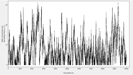
The M/M/1 queue process is characterized by a short warm-up period. However, the process
ex-hibits a strong autocorrelation structure, with the autocorrelation function for the waiting time lags
decaying slowly with increasing lags. Also, theM/M/1 queue waiting times have a steady-state
proba-bility distribution which has a nonzero probaproba-bility at zero and a exponential tail. This results in a slow
convergence of the batch means to the normal distribution with increasing batch size.
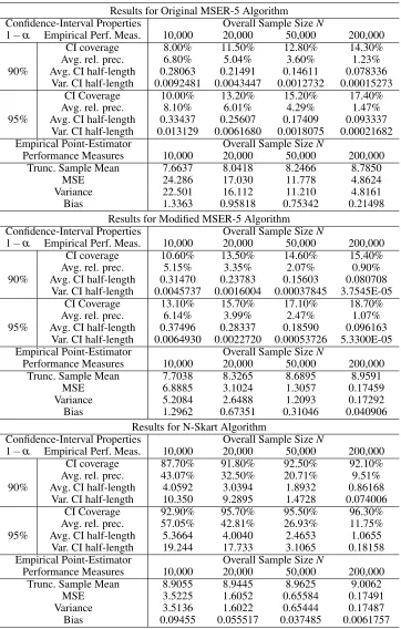
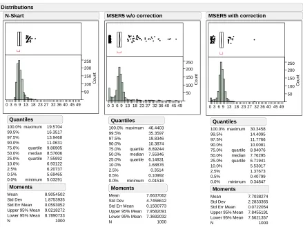
Figure 3.1 depicts a single realization of the first M/M/1 queue-waiting-time process. Table 3.1
summarizes the performance of the original MSER-5 algorithm, the modified MSER-5 algorithm, and
N-Skart on 1,000 independent replications of this test process. Figures 3.2—3.5 display the empirical
Table 3.1: Performance of MSER-5 and N-Skart in theM/M/1 queue-waiting-time process with 90% server utilization and empty-and-idle initial condition
Results for Original MSER-5 Algorithm
Confidence-Interval Properties Overall Sample SizeN
1−α Empirical Perf. Meas. 10,000 20,000 50,000 200,000
CI coverage 8.00% 11.50% 12.80% 14.30%
Avg. rel. prec. 6.80% 5.04% 3.60% 1.23%
90% Avg. CI half-length 0.28063 0.21491 0.14611 0.078336
Var. CI half-length 0.0092481 0.0043447 0.0012732 0.00015273
CI Coverage 10.00% 13.20% 15.20% 17.40%
Avg. rel. prec. 8.10% 6.01% 4.29% 1.47%
95% Avg. CI half-length 0.33437 0.25607 0.17409 0.093337
Var. CI half-length 0.013129 0.0061680 0.0018075 0.00021682
Empirical Point-Estimator Overall Sample SizeN
Performance Measures 10,000 20,000 50,000 200,000
Trunc. Sample Mean 7.6637 8.0418 8.2466 8.7850
MSE 24.286 17.030 11.778 4.8624
Variance 22.501 16.112 11.210 4.8161
Bias 1.3363 0.95818 0.75342 0.21498
Results for Modified MSER-5 Algorithm
Confidence-Interval Properties Overall Sample SizeN
1−α Empirical Perf. Meas. 10,000 20,000 50,000 200,000
CI coverage 10.60% 13.50% 14.60% 15.40%
Avg. rel. prec. 5.15% 3.35% 2.07% 0.90%
90% Avg. CI half-length 0.31470 0.23783 0.15603 0.080708
Var. CI half-length 0.0045737 0.0016004 0.00037845 3.7545E-05
CI Coverage 13.10% 15.70% 17.10% 18.70%
Avg. rel. prec. 6.14% 3.99% 2.47% 1.07%
95% Avg. CI half-length 0.37496 0.28337 0.18590 0.096163
Var. CI half-length 0.0064930 0.0022720 0.00053726 5.3300E-05
Empirical Point-Estimator Overall Sample SizeN
Performance Measures 10,000 20,000 50,000 200,000
Trunc. Sample Mean 7.7038 8.3265 8.6895 8.9591
MSE 6.8885 3.1024 1.3057 0.17459
Variance 5.2084 2.6488 1.2093 0.17292
Bias 1.2962 0.67351 0.31046 0.040906
Results for N-Skart Algorithm
Confidence-Interval Properties Overall Sample SizeN
1−α Empirical Perf. Meas. 10,000 20,000 50,000 200,000
CI coverage 87.70% 91.80% 92.50% 92.10%
Avg. rel. prec. 43.07% 32.50% 20.71% 9.51%
90% Avg. CI half-length 4.0592 3.0394 1.8932 0.86168
Var. CI half-length 10.350 9.2895 1.4728 0.074006
CI Coverage 92.90% 95.70% 95.50% 96.30%
Avg. rel. prec. 57.05% 42.81% 26.93% 11.75%
95% Avg. CI half-length 5.3664 4.0040 2.4653 1.0655
Var. CI half-length 19.244 17.733 3.1065 0.18158
Empirical Point-Estimator Overall Sample SizeN
Performance Measures 10,000 20,000 50,000 200,000
Trunc. Sample Mean 8.9055 8.9445 8.9625 9.0062
MSE 3.5225 1.6052 0.65584 0.17491
Variance 3.5136 1.6022 0.65444 0.17487
Report: mm1e91 Page 1 of 1 50 100 150 200 250 Count
0 3 6 9 13 18 23 27 32 36 40 45 49
100.0% 99.5% 97.5% 90.0% 75.0% 50.0% 25.0% 10.0% 2.5% 0.5% 0.0% maximum quartile median quartile minimum 19.5704 16.3517 13.9468 11.0631 9.86905 8.57606 7.55992 6.93122 6.20737 5.69465 5.03291 Quantiles Mean Std Dev Std Err Mean Upper 95% Mean Lower 95% Mean N 8.9054502 1.8753935 0.0593052 9.0218272 8.7890733 1000 Moments N-Skart 50 100 150 200 250 Count
0 3 6 9 13 18 23 27 32 36 40 45 49
100.0% 99.5% 97.5% 90.0% 75.0% 50.0% 25.0% 10.0% 2.5% 0.5% 0.0% maximum quartile median quartile minimum 46.4403 35.3597 19.8346 10.3874 8.89244 7.55946 6.14831 1.68876 0.3514 0.10992 0.01516 Quantiles Mean Std Dev Std Err Mean Upper 95% Mean Lower 95% Mean N 7.6637062 4.7458612 0.1500773 7.9582091 7.3692032 1000 Moments
MSER5 w/o correction
50 100 150 200 250 Count
0 3 6 9 13 18 23 27 32 36 40 45 49
100.0% 99.5% 97.5% 90.0% 75.0% 50.0% 25.0% 10.0% 2.5% 0.5% 0.0% maximum quartile median quartile minimum 30.3458 14.4095 11.7766 10.0081 8.94076 7.76295 6.71941 5.53017 1.37673 0.40799 0.34847 Quantiles Mean Std Dev Std Err Mean Upper 95% Mean Lower 95% Mean N 7.7038274 2.2833365 0.0722054 7.8455191 7.5621357 1000 Moments
MSER5 with correction Distributions
Figure 3.2: Empirical distributions of truncated sample mean for N-Skart, MSER-5, and modified
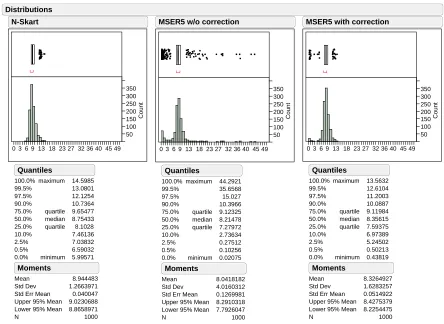
Report: mm1e92 Page 1 of 1 50 100 150 200 250 300 350 Count
0 3 6 9 13 18 23 27 32 36 40 45 49
100.0% 99.5% 97.5% 90.0% 75.0% 50.0% 25.0% 10.0% 2.5% 0.5% 0.0% maximum quartile median quartile minimum 14.5985 13.0801 12.1254 10.7364 9.65477 8.75433 8.1028 7.46136 7.03832 6.59032 5.99571 Quantiles Mean Std Dev Std Err Mean Upper 95% Mean Lower 95% Mean N 8.944483 1.2663971 0.040047 9.0230688 8.8658971 1000 Moments N-Skart 50 100 150 200 250 300 350 Count
0 3 6 9 13 18 23 27 32 36 40 45 49
100.0% 99.5% 97.5% 90.0% 75.0% 50.0% 25.0% 10.0% 2.5% 0.5% 0.0% maximum quartile median quartile minimum 44.2921 35.6568 15.027 10.3966 9.12325 8.21478 7.27972 2.73634 0.27512 0.10256 0.02075 Quantiles Mean Std Dev Std Err Mean Upper 95% Mean Lower 95% Mean N 8.0418182 4.0160312 0.1269981 8.2910318 7.7926047 1000 Moments
MSER5 w/o correction
50 100 150 200 250 300 350 Count
0 3 6 9 13 18 23 27 32 36 40 45 49
100.0% 99.5% 97.5% 90.0% 75.0% 50.0% 25.0% 10.0% 2.5% 0.5% 0.0% maximum quartile median quartile minimum 13.5632 12.6104 11.2003 10.0887 9.11984 8.35615 7.59375 6.97389 5.24502 0.50213 0.43819 Quantiles Mean Std Dev Std Err Mean Upper 95% Mean Lower 95% Mean N 8.3264927 1.6283257 0.0514922 8.4275379 8.2254475 1000 Moments
MSER5 with correction Distributions
Figure 3.3: Empirical distributions of truncated sample mean for N-Skart, MSER-5, and modified
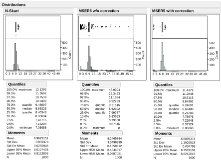
Report: mm1e93 Page 1 of 1 100 200 300 400 500 Count
0 3 6 9 13 18 23 27 32 36 40 45 49
100.0% 99.5% 97.5% 90.0% 75.0% 50.0% 25.0% 10.0% 2.5% 0.5% 0.0% maximum quartile median quartile minimum 12.1292 11.3692 10.7538 10.0399 9.43607 8.89226 8.40343 8.00604 7.47716 7.13204 7.05056 Quantiles Mean Std Dev Std Err Mean Upper 95% Mean Lower 95% Mean N 8.9625151 0.809379 0.0255948 9.0127408 8.9122893 1000 Moments N-Skart 100 200 300 400 500 Count
0 3 6 9 13 18 23 27 32 36 40 45 49
100.0% 99.5% 97.5% 90.0% 75.0% 50.0% 25.0% 10.0% 2.5% 0.5% 0.0% maximum quartile median quartile minimum 45.9204 29.3463 11.1684 9.92293 9.21515 8.62302 7.99787 5.83653 0.29858 0.07516 0 Quantiles Mean Std Dev Std Err Mean Upper 95% Mean Lower 95% Mean N 8.2465784 3.3498399 0.1059312 8.4544517 8.0387051 1000 Moments
MSER5 w/o correction
100 200 300 400 500 Count
0 3 6 9 13 18 23 27 32 36 40 45 49
100.0% 99.5% 97.5% 90.0% 75.0% 50.0% 25.0% 10.0% 2.5% 0.5% 0.0% maximum quartile median quartile minimum 11.4379 11.2648 10.5115 9.84991 9.24691 8.69489 8.21203 7.75676 7.22648 0.37329 0.06868 Quantiles Mean Std Dev Std Err Mean Upper 95% Mean Lower 95% Mean N 8.6895374 1.1002515 0.034793 8.7578132 8.6212616 1000 Moments
MSER5 with correction Distributions
Figure 3.4: Empirical distributions of truncated sample mean for N-Skart, MSER-5, and modified
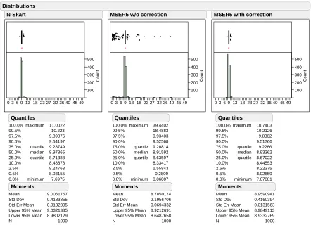
Report: mm1e94 Page 1 of 1 100 200 300 400 500 Count
0 3 6 9 13 18 23 27 32 36 40 45 49
100.0% 99.5% 97.5% 90.0% 75.0% 50.0% 25.0% 10.0% 2.5% 0.5% 0.0% maximum quartile median quartile minimum 11.0022 10.223 9.89076 9.54197 9.28749 8.97865 8.71388 8.48878 8.24763 8.03155 7.6975 Quantiles Mean Std Dev Std Err Mean Upper 95% Mean Lower 95% Mean N 9.0061757 0.4183855 0.0132305 9.0321385 8.9802129 1000 Moments N-Skart 100 200 300 400 500 Count
0 3 6 9 13 18 23 27 32 36 40 45 49
100.0% 99.5% 97.5% 90.0% 75.0% 50.0% 25.0% 10.0% 2.5% 0.5% 0.0% maximum quartile median quartile minimum 39.4402 18.4883 9.93403 9.52568 9.20814 8.91592 8.63597 8.33417 1.55843 0.2809 0.06007 Quantiles Mean Std Dev Std Err Mean Upper 95% Mean Lower 95% Mean N 8.7850174 2.1956706 0.0694332 8.9212691 8.6487658 1000 Moments
MSER5 w/o correction
100 200 300 400 500 Count
0 3 6 9 13 18 23 27 32 36 40 45 49
100.0% 99.5% 97.5% 90.0% 75.0% 50.0% 25.0% 10.0% 2.5% 0.5% 0.0% maximum quartile median quartile minimum 10.7403 10.2126 9.8362 9.51766 9.2266 8.93362 8.67022 8.44553 8.22375 8.02859 7.67081 Quantiles Mean Std Dev Std Err Mean Upper 95% Mean Lower 95% Mean N 8.9590941 0.4160394 0.0131563 8.9849113 8.9332769 1000 Moments
MSER5 with correction Distributions
Figure 3.5: Empirical distributions of truncated sample mean for N-Skart, MSER-5, and modified
Consider the results forM/M/1 queue with 90% server utilization and empty and idle initial
con-dition. The steady-state mean of this process is 9.0. From the results in Table 3.1, it is evident that
the confidence-interval properties obtained from N-Skart were considerably better than those obtained from both the MSER-5 algorithms. The confidence interval coverages delivered by N-Skart were
ex-tremely close to the specified coverages. For smaller sample sizes, N-Skart delivered results with lesser
CI coverages than specified; but it also delivered a CI with wider relative precision, indicating that a larger sample size was required in order to have practically useful CIs. As the sample size increased,
N-Skart delivered CI estimates close to the specified coverage and in most cases, the actual coverage
was better than the specified CI coverage as is observed in the case of sample size 200,000 and specified coverage of 95%. As against this, the CI delivered by both the MSER-5 algorithms exhibited very low
CI coverages, typically in the range 10%−20%. The average relative precision and the actual CI
half-length delivered by N-Skart was almost an order of magnitude higher than that delivered by MSER-5, which indicates that in addition to providing a valid CI for the point estimator, N-Skart also provides a
much more realistic estimate of the true precision of the truncated sample mean (as measured by the CI relative precision or the CI average half-length) than either version of MSER-5 provides.
While considering the point estimator delivered by both the methods, it was observed that the
MSER-5 algorithms greatly underestimated the value of the steady-state mean. The MSE and vari-ance in the estimate of the steady-state mean was at least an order of magnitude smaller for N-Skart
than MSER-5, for all sample sizes. The modified MSER-5 provided improved results over the original
MSER-5 by reducing the MSE by an order of magnitude for smaller sample sizes, but these values were still substantially larger than those delivered by N-Skart. Another point worth mentioning here is that
for both N-Skart and MSER-5, the variance was the main contributor in the MSE.
The bias and variance in the estimate of the steady-state mean can also be observed in the histograms depicted in Figures 3.2—3.5. The truncated sample means were distributed over a much wider range
in the case of both the MSER-5 algorithms. Also, for smaller sample sizes, the distribution exhibited
bimodal characteristics, and the mode was shifted to the left of the distribution. It was also observed
that MSER-5 delivered mean estimates as high as 46.44, which is completely unrepresentative of the
steady-state mean of this test process. Moreover, for sample size 10,000, the upper and lower quartiles
3.2.2. M/M/1 Queue-Waiting-Time Process with Empty Initial Condition and 80% Uti-lization
This test process is similar to the first test process but the interarrival times are sampled from an
ex-ponential distribution with an arrival rate of λ =0.8 arrivals per unit time. The steady-state server
utilization for this process is given by
ρ=λ
µ =
0.8
1.0=0.8. (3.4)
The system starts in the empty-and-idle state so thatX1=0 on every replication of the process {Xj}.
Thus, the steady-state expected waiting time for this process is given by
µX =lim
j→∞
E(Xj)
ρ
1−ρ =4.0 time units (3.5)
Figure 3.6 depicts a single realization of theM/M/1 queue-waiting-time process with empty-and-idle
initial condition and 80% server utilization. Table 3.2 summarizes the performance of MSER-5,
mod-ified MSER-5, and N-Skart on 1,000 independent replications of this test process. Figures 3.7—3.10
display the empirical distributions of the truncated sample mean delivered by all three procedures in this test process. The results for this process are given below.
Figure 3.6: A realization of theM/M/1 queue-waiting-time process with empty-and-idle initial