Simplified Estimation Method for First Excursion Probability of Secondary System with Hysteresis Characteristics

(1)

Simplified Estimation Method for First Excursion Probability of Secondary System with

Hysteresis Characteristics

Shigeru Aoki 1)

1)Department of Mechanical Engineering, Tokyo Metropolitan College of Technology, Higashi-Ohi, Shinagawa-ku, Tokyo, Japan

ABSTRACT

When the secondary system such as pipings, tanks and other mechanical equipment installed on the primary system such as buildings is subjected to excess seismic load, the response of the system exceeds yield deformation. In this paper, an simplified estimation method of the first excursion probability of the secondary system with hysteresis loop characteristics caused by plastic deformation is proposed. As an analytical model, the primary system and the secondary system are simulated as single-degree-of-freedom system respectively for simplicity. As restoring force-deformation relation, bilinear hysteresis loop characteristics is used. First, an analytical method for the secondary system with hysteresis loop characteristics caused by plastic deformation is presented. This method is based on equivalent linearization method. As input excitations, two kinds of artificial time histories are used. One is nonstationary filtered white noise and the other is artificial time history compatible to the design response spectrum. Next, by using the proposed method, some numerical examples are shown. From the numerical examples, it is found that when the tolerance level is normalized by the maximum response or the maximum standard deviation of response of the linear secondary system without plastic deformation, the first excursion probability is independent of mass ratio of the secondary system to the primary system, the damping ratio and the natural period of the sexondary system. For aseismic design of structures, response spectrum which corresponds to the maximum response of the single-degree-of-freedom system is used. The maximum response of the secondary system can be estimated by amplification factor or modal analysis. The maximum standard deviation corresponds to the maximum response. The proposed method is expected to be practical and simplified estimation method of the first excursion probability of the secondary system.

INTRODUCTION

Mechanical structures such as pipings, tanks and other mechanical equipment are usually installed on supporting structures such as buildings. Mechanical structures are referred to as the secondary systems. Supporting structures are referred to as the primary systems. In the case of earthquake, the secondary system is subjected to seismic excitation through the primary system. When the natural period of the secondary system is close to that of the primary system, the response of the secondary system is greatly amplified[i]. The response of the secondary system exc.ee_,ds elastic limit when the secondary system is subjected to excess seismic loading[2]. In this case, restoring force-deformation relation is modeled as hysteresis loop characteristics.

In aseismic design, response spectrum which is the maximum response of single-degree-of-freedom system is used[3]. For the secondary system, the floor response spectrum which is the maximum response of the secondary system usually used[4]. The important secondary system should be designed so as to maintain its function during and after seismic loading. Some failure modes are seen. First excursion failure is one of the most important failure modes. It is pointed out that safety of the important secondary system is evaluated in probabilistic manner[5]. Thus, first excursion probability is one of the most important safety factors.

In this paper, a simplified estimation method of first excursion probability of the secondary system with hysteresis loop characteristics caused by plastic deformation is proposed. For simplicity, the primary system and the secondary system are simulated as single-degree-of-freedom system respectively. Many models of hysteresis loop characteristics are proposed. In this paper, bilinear hysteresis loop characteristics is used. First, an analytical method for first excursion probability of the secondary system with hysteresis loop characteristics is presented. First excursion probability is obtained by using moment equations. This method is based on equivalent lineafization method. As input excitations, two kinds of artificial time histories are used. One is nonstationary filtered white noise and the other is artificial time history compatible to the design response spectrum. Next, by using the proposed method, some numerical examples are shown. From the numerical examples, it is found that when the tolerance level is normalized by the maximum response or the maximum standard deviation of response of the linear secondary system without plastic deformation, the first excursion probability is independent of mass ratio of the secondary system to the primary system, the damping ratio and the natural period of the secondary system. For aseismic design of structures, response spectrum which corresponds to the maximum response of the single-degree-of-freedom system is used. The maximum response of the secondary system can be estimated by amplification factor or modal analysis[i][4]. The maximum standard deviation corresponds to the maximum response[6]. The proposed method is expected to be practical and simplified estimation method of the first excursion probability of the secondary system.

ANALYTICAL M O D E L AND INPUT EXCITATIONS

Actual secondary system is complex and sometimes modeled as multi-degree-of-freedom system. In this paper, in order to obtain basic properties of first excursion probability, the secondary system and the primary system are simulated as single-degree-of-freedom system for simplicity. Figure 1 shows an analytical model used in this study. Spring element of the secondary system is assumed to have bilinear hysteresis loop characteristics. Equations of motion of the model are expressed as:

SMiRT 16, Washington DC, August 2001 Paper # 1049

(2)

Zs + 2~smsZs + f = -Zs - Y

}

Zp + 2~pO)pZp + O.)p2Zp-

~,(2~sms~: s + f ) = - ~ )

0)

where z s is relative displacement of the secondary system to the primary system x s

- Xp, Zp

is relative displacement of the primary system to the ground Xp - y. ~s (- cs / 2x/msk s ) and ~p (- Cp / 2~/mpkp ) are the damping ratio of the secondary system and the primary system, respectively, m s (- x/ks / m s ) and O)p (- 4kp / mp ) are the natural circular fl'equency of the secondary system and the primary system, respectively. ~, is mass ratio of the secondary system to the primary system, f is nonlinear restoring force in the secondary system. ~; is input excitation.

As input excitations, two kinds of artificial time histories are used. One is nonstationary filtered white noise. The other is artificial time histories compatible to design response spectrum. Figure 2 shows envelope function I(t) for nonstationary filtered white noise. Figure 3 and Figure 4 show target response spectrum[7] and envelope function I(t)[8] for artificial time history compatible to design response spectrum. Power spectral density function of ground motion is given as[9]"

(2~g(DgO)) 2 + (Dg 4

G(°)) = ((Og 2 0)2 )2 + (2 ~ g (,O g O) )2

Go

(2)

where ~ and m

_g

are the damping ratio and the natural circular frequency of the ground model. G0 is power spectral density of white noise which simulates base rock motion. For artificial time history, ~g =0.5, Tg(-2~t/mg)=0.285s and G0-1.94x103(1/s)[9]. Equations of motion of the ground model is given as:

= I(t)(Zg + ~}g) ]

(3)

Zg + 2~g0JgZg + 0.)g2Zg =--yg

where Z g is relative displacement of ground to base rock and ~ g is acceleration of base rock.

THEORETICAL METHOD FOR FIRST EXCURSION PROBABII JTY

It is assumed that the secondary system fails when absolute value of relative displacement z s first crosses the tolerance level B D . First excursion probability is obtained by the following equation.

Pf(t) = 1 - e x p { - 2 ~ v(t)dt}

(4)

When instants at which z s crosses B D are statistically independent, v(t) is given as:

[{

( )

v ( t ) - 1 ~ exp - BD2 1+ ZsZ s +BDKz,~ ~ a; exp - BD2 {[

2

2ax 0"Zs 20"z~ 2 D 2D0"z~ 20"z, 2

+ erf (C)}]

(5)

2

where 0"z is variance of relative displacement of the secondary system, 0"~, of relative ctisplacement and relative velocity. And,

2 °

is variance of relative velocity and KZ~is is covariance

KZsZs

20".2

eft(u) 2-~-f0u (_

2~

C = ,D=0"zs Zs -KZ?s, = exp y y (6)

2D0"zs

(3)

--=0P

0p k + 2~pmpp- 0p ~2~pmpZ - COp2Zp+y(2~smsZs +f)+ I(t)(2~gmgzg +mg2Zg)}

Ot - OZp p ~Zp P

Op i .

{- 2~smsk s (1 + Y)Zs -(1+ y)f + 2~pmp~p +

Zp t

",t

0p Zs + 2~smsZs (1 + y ) p - - ~ z s

0)p 2

0z s

0__pp (9

)+ 02p a-G°

0p

Zg +

2~gO3gp

+ W~gO.)gZg + 038

0Zg 0Zg 2Zg 0~g 2 2

where f is restoring force in the secondary system, f is equvalently linearized as follows.

(7)

2

f

= 2~eqO)eqZ s + OJeq Z s (8)

2 2

where

~eq iS equivalent damping ration and C0eq is equivalent natural circular frequency. In order to use Eq.(4), OZs., O~s and

KZs~. s are to be obtained. Applying the partal integral method to Eq.(7), moment equations with respect to z s , Zs, Zp, Zp, Zg and

~g are obtained as follows:

00" z 2 _p

0t

0KZpZs

0t

0KZp2;p

0t

0KZp~ s

0t

--. 2Kzpkp

-- K~pZs + KZp~: s

2 2 0 2 _2~p0JpK + (2~sm s +

2~e q

~ K Z p

I(T)KzpZg

+ 2~gmgI(t)KZpeg

--" Orkp -- O)p Zp + O)eq2~tKzpzs ZpZp O)eq ~-s + O)g 2

Kkpks + 0.)p2OZp 2 2(1+ ~t)Kzpzs + (2~s0Js +

~1+

)K:

= -- (Deq 2~p(1)pKzpkp -- 2~eq0)eq Y Zp2; s

0KZpZg

0t -- K~;pZg "[" Kzp~:g

0Kzp7,g

0t

0(jz s 2

0t

0K2:pZ s

0t

--" K~p~g -- 0)g2K _ZpZg--

2~g

_('0gKZpZg

= 2KZs~

KZP ~s _ (.0p2K 2

= ZpZs + O)eq2~OZs

-2~pmpKipZs + (2~sC0 s + 2~eqmeq ~KZs~.s + C0g2I(t)KZsZg + 2~pmpI(t)KZs~g

OKz~. s

0t

2 2 0 + 7)OZs 2

-- (JZs + O~p2Kz _pZs- O.)eq + 2~pC0pK ~pZs --(2~s0) s + 2~eq0keq ~1 + ]t)Kzs~s

OKZ~Zg

ot = K~.sZg + KZs~:g

0KZs~g

(4)

-

2 0)p2K

.

2 + C0g2I(T)K2

+ 2~gO)gi(t)Kkpig

0 t

ZPZs + (DeqgYKzPZs -- 2¢p0~pO7"s +

(2¢sms

+ 2¢eq0~eq ~K~p~s

pZg

0K 2;p~; s

0t

-- O)p

2

KZp~s

+

0.)eq2~Kzsks - 2~p0)pKkpks

+ (2~s0ks + 2~eq0Jeq ~Oks 2 + O)g2I(t)Kk#g

+0)p2K .

ZpZp f'Oeq 2

__ ( l + 7 ~ p Z s

+ 2~p0JpCr~p 2 (2~s0ks + 2~eq0)eq ~1 + Y ~gpk s

2

+ 2~gmgI(t)l~s~.g

0Kzpzg

0t -- --O)p2KZpZg

+

K~;p~g

+

(Deq2~tKzszg -- 2~p0kpK~pzg + (2~s0)s + 2~eq0)eq~Kkszg + 0)g2I(t)OZg 2 + 2~gO)gI(t)Kzg~,g

0]~.p~g = --C0p2Kzpzg. + O)eq2]tKzs/g - 2~p0)pK).pig + (2~sO)s + 2~eq0Jeq ~K~.skg +

C°g2I(t)KZgkg + 2~gmgI(t)°~g 2

2

-

(0g K~pZg -- 2~g(0gK~;p~g

0t

OOZs2 _ 2 ~ p 2 K

_0t

. _

2(l+~Zs~s +2~p0)pK~p~, s -(2~s0)s + 2 ~ e q 0 k e q ~ l + ~ g

2}

ZPZs

0)eq

0K7,sZg

0t --

0~p2K

ZpZg -- ('0eq

20 -I- ?~(ZsZg +

2~p0)pK~.pZg --

(2~s(20s +

2~eqO)eq

)(1"[" ~(~.s z "{-

? g

KZsZg

0KZs7g

_

2 K .

0 t

= 02p2 KZp~g -- ~eq2(1 + ~Zs~g -l- 2~pf0pK~p~,g --

(2~ sco s

+ 2~e q0)eq

~1

+ ~ , s ~ g

O)g ZsZg - 2~g0~gK~,s~,g

00

2

Zg

0t

-- 2Kzg~g

0KZgZg

0t

2

2 --

(~Zg --

~-~ Q~g

(0g

2~g(0gKzg2g

0t -2(-mgZKzgig

- 2~gmgOig 2)+ a~G0

(9)

Solving moment equations(8) and using Eqs.(5) and (6), first excursion probability is obtained from Eq.(4).

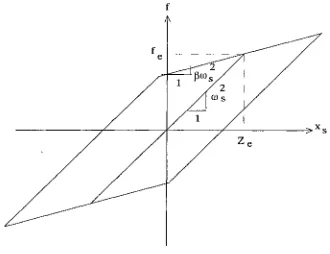
N O ~ CHARACTERISTICS

As nonlinear characteristics, bilinear hystersis loop characteristics as shown in Fig.5 is used. f~ is yield force and [3 is ratio of post-yield stiffness to pre-yield stiffness. Restoring force f is equivalently linearized as Eq.(8). When nonlinear effect is not so great, it is assumed that the effect of yield is great near the main shock. It is also assumed that z s (t) near the main shock is stationary random process and its distribution of amplitude is the Rayleigh distribution. ~eq and C%q are obtained by stationary random process theory as follows.

_

COs2erfc(Tl-a ~1 - [3)

[

h e

-

%/~-(De2TI

(10)

O)e 2 =(Ds 2

- O~s2 ~xp(- n-2)- n-l,,/~erfc(~-a)il- 13)} ]

(5)

erfc(u) = 1 - ~ f 0 u exp(- v2 )iv, rl = x[2OZs / Ze (11)

For the system with hysteresis loop Characteristics caused by ~lastic deformation, yield force is normalized by the maximum standard

. . . . 2

deviation ofrestonng force of the elastic secondary system m s lOse[max as fOllOWS.

~ = fe/ms2l%e[max (12)

The tolerance level

BD

is normalized by the maximum standard deviation of relative displacement of the elastic secondary system

lose

[max as follows.

at = BD/los~

Imax

(13)

The maximum standard deviation corresponds to the maximum response[6]. The maximum response of the secondary system can be estimated by amplification factor or modal analysis[ 1][4].

NUMERICAL EXAMPLF~

From Eq.(4), the first excursion probability p f is function of time t. Important secondary system should maintain their function after earthquake excitation decays. Hence, p f at the end of earthquake excitation is obtained. Since many parameters are determined, values of some parameters are fixed. The damping ratio of the primary system is fixed as 0.05. The natural period of the secondary system

T s (2z~ / m s ) coincide with that of the primary system Tp (2zc / (Dp ~, SinCe response of the segondary system is greatly amplified.

From Table 1 to Table 6, results for nonstationna/3, filtered white noise excitations are shown. Table 1, Table 2 and Table 3 show results for c~=1.0 and [3--0. In this case, hysteresis loop has peffectly-elasto-plastic charactereistics. Table 1 shows p f for some valus of mass ratio T. Table 2 shows p f for some values of the damping ratio of the secondary system ~s. Table 3 shows pf for some values of the natural period of the ~condary system T s and that of the primary system Tp. Form Table 1, p f becomes large when ~, increases. However, variation of pf is not so great. From Table 2, pf becomes large when ~s increases. However, variation of pf is small. From Table 3, pf bea3mes large when T s and Tp becomes short. However, variation of pf is small.

Table 4, Table 5 and Table 6 show results for a=l.0 and [3---0.5. In this case, hysteresis loop has bilinear hysteresis loop charactereistics. Table 4 shows p f for some valus of mass ratio y. Table 5 shows p f for some values of the damping ratio of the secondary system 7~ s . Table 6 shows pf for some values of the natural period of the secondary system T s and that of the primary system Tp. Form Table 4, p f becomes large when ~, increases. However, variation of p f is not so great. From Table 5, p f becomes large when ~s increases. However, variation of pf is small. From Table 6, pf becomes large when T s and Tp becomes short. However, variation of pf is small.

From Table 7 to Table 9, results for nonstationnary filtered white noise excitations are shown. Table 7, Table 8 and Table 9 show results for a=l.0 and [3--0. In this case, hysteresis loop has perfectly-elasto-plastic charactereistics. Table 7 shows p f for some valus of mass ratio y. Table 8 shows p f for some values of the damping ratio of the secondary system ~s- Table 9 shows p f for some values of the natural period of the secondary system T s and that of the primary system Tp. Form Table 7, p f becomes large when ~, increases. However, variation of p f is not so great. From Table 8, p f becomes large when ~s increases. However, variation of p f is small. From Table 9, p f becomes large when T s and Tp becomes short. However, variation of p f is small.

CONCLUSIONS

A simplified estimation method for the first excursion probability of the secondary system with hysteresis characteristics caused by plastic deformation is examined. As input excitations, nonstationary filtered white noise and artificial time history compatible to the design response spectrum are used. When the tolerance level is normalized by the maximum standard deviation of the secondary system without nonlinear characteristics as Fq.(13). variation of the first excursion probability is not so great independent of mass ratio of the secondary system to the primary system, the damping ratio and the natural period of the secondary system and the primary system. The maximum standard deviation corresponds to the maximum response. Hence, the proposed method is expected to be practical and simplified estimation method of the first excursion probability of the secondary system.

REFERENCES

1. Suzuki,K. and Aoki, S., "Conventional Estimating Method of Earthquake Response of Mechanical Appendage System Installed in the Nuclear Structural Facilities", Trans of 6th SMiRT, K10/3, 1981

(6)

3. Hart, G.C. and Wong, K., Structural Dynamics for Structural Engineers, John Wiley & Sons, 1999 4. Gupta,A.J., Response Spectrum Method, Blackwekk Scientific Publication, 1990

5. Lin,Y.K. and Cai,G.Q., Probabilistic Structural Dynamics, MacGraw-Hill, 1995

6. Tajimi, H., "A Statistical Method of Determining the Maximum Response of a Building Structure during an Earthquake", Proc. of 2WCEE, Vol.II, 1960, pp.781-798

7. Japanese Ministry of International Trade and Industry, Guidelines for Aseismic Design of High Pressure Gas Facilities, 1983

8. Jennings,EC. et al., "Simulated Earthquake Motions", Earthquake Engineering Research Laboratory, California Institute of Technology, 1968

9. Aoki,S. and Suzuki, K., "First Excursion Probability Estimation of Mechanical Appendage System Subjected to Nonstationary Earthquake Excitations", Proc. of 4th ICOSSAR, 1985, pp.201-210

0.8 m s

I C s

m p

k lp ICp

F

x

{

x _p

t

Fig.1 Analytical model of secondary system

0.6

0.4 0.2

0.8 I(t)

e - O . 1 2 5 t _ e - 0 . 2 5 t

tlmax

I I I I I I

0 5 10 15 20 25 30

' t(s) 35

Fig.2 Envelope function for nonstationary filtered white noise

0 . 5

/

\

0 . 0 5 0 . 1 0 . 5 1 5

N a t u r a l P e r i o d ( s )

Fig.3 Target response spectrum for artificial time history

I(t) A

0.6

0.4

0.2

B

OA:i(t)=t2/16 A B :I(t)= 1.0

B C :I(t)= exp { -0.0924(t-15~}

; = . . -

0 10 20 30 40 50

(7)

f

f . . . .

s

Fig.5 Bilinear restoring force-deformation relation

Table i

(~t

1.5 2.0 2.5 3.0

First excursion probability of secondary system for nonstationary filtered white noise (~s = 0.01, T s = 0.5s, ~p = 0.05, Tp = 0.5s, ~g = 0.4, Tg = 0.5s, ot = 1,13 = 0)

0 0.969 0.527 0.114 0.014

0.01

7

0.02 0.05 0.1

0.996 0.999 1.000 1.000 0.842 0.927 0.979 0.992 0.397 0.581 0.803 0.906 0.105 0.214 0.449 0.645

Table 2 First excursion probability of secondary system for nonstationary filtered white noise (y = 0, T s = 0.5s, ~p --- 0.05, Tp -- 0.5s, ~g -- 0.4, Tg --- 0.5s, ot -- 1,13 -- 0)

6t 1.5 2.0 2.5 3.0

~S

0.01 0.02 0.05 0.1

0.969 0,964 0.977 0.987 0.527 0.526 0.613 0.712 0.114 0.118 0.165 0.240

0.014 0.016 0.025 0.045

Table 3 First excursion probability of secondary system for nonstatinary filtered white noise (y - 0, ~s = 0.01, ~p - 0.05, T s - T p , ~ g - 0.4, T g - 0 . 5 s , ot - 1, [3 - 0)

6t 1.5 2.0 2.5 3.0

Ts--rp

0.3s 0.5s 0.8s 1.0s

0.997 0.969 0.917 0.892 0.745 0.527 0.429 0.409 0.210 0.114 0.093 0.093 0.029 0.014 0.013 0.014

Table 4

(~t

1.5 2.0 2.5 3.0

First excursion probability of secondary system for nonstationary filtered white noise (~s = 0.01, T s = 0.5s, ~p = 0.05, Tp = 0.5s, ~g = 0.4, Tg = 0.5s, ot = 1, [3 = 0.5)

Y

0 0.01 0.02 0.05 0.1

(8)

Table 5 First excursion probability of secondary system for nonstationary filtered white noise

(It = 0, r s --" 0 . 5 s , ~p = 0 . 0 5 , Tp -- 0.5s, ~g - 0.4, Zg -- 0.5s, 12 -- 1, ~ = 0 . 5 )

1.5 2.0 2.5 3.0

~S

0.01 0.02 0.05 0.1

0.995 0.992 0.993 0.994 0.784 0.757 0.779 0.809 0.294 0.281 0.311 0.350 0.060 0.059 0.070 0.085

Table 6 First excursion probability of secondary system for nonstationary filtered white noise

(It = 0, ~s --- 0 . 0 5 , ~p = 0 . 0 5 , Z s = Tp, ~g = 0.4, Tg = 0.5s, 12 --- 1, [~ - 0 . 5 )

a t

1.5 2.0 2.5 3.0

Ts-T

0.3s 0.5s 0.8s 1.Os

1.0(03 0.995 0.981 0.972 0.922 0.784 0.686 0.689 0.455 0.294 0.237 0.228 0.108 0.060 0.049 0.048

Table 7 First excursion probability of secondary system for artificial time history (~s = 0.01, T s - 0.5s, ~p = 0.05, Tp - 0.5s, ~g ---- 0.5, Tg -- 0.285s, 12 = 1, [3 - 0)

1.5

2.0

2.5 3.0

0 0.01

0.987 0.998 0.599 0.957 0.124 0.600 0.013

0.02 0.05 0.1

1.000 1.0t30 1.(K)0 0.988 0.999 0.988 0.790 0.946 0.817

0.682

0.190 0.367 0.434

Table 8 First excursion probability of secondary system for artificial time history (7 - 0, T s = 0.5s, ~p - 0.05, Tp -- 0.5s, ~g = 0.5, Tg -- 0.285s, 12 = 1, [5 = 0)

~t

1.5 2.0 2.5 3.0

~S

0.01 0.02 0.05 0.1

0.987 0.991 0.997 0.999 0.599 0.654 0.798 0.896 0.124 0.155 0.271 0.417 0.013 0.019 0.044 0.084

Table 9 First excursion probability of secondary system for artificial time history (y = 0, ~s = 0.01, ~p = 0.05, T s = Tp, ~g = 0.5, Tg = 0.285s, 12 = 1 [3 = 0)

6t 1.5 2.0 2.5 3.0

0.3s 0.5s 0.8s 1.0s