Structural Breaks, Model Selection, and Overidentification in Dynamic Factor Models.

(1)

ABSTRACT

HAN, XU. Structural Breaks, Model Selection, and Overidentification in Dynamic Factor Models. (Under the direction of Dr. Atsushi Inoue.)

The first chapter develops tests for structural breaks of factor loadings in dynamic factor

models. We focus on the joint null hypothesis that all factor loadings are constant over time.

Because the number of factor loading parameters goes to infinity as the sample size grows, the

conventional test cannot be used. Based on the fact that the estimated factors will demonstrate

a higher dimension under the alternative hypothesis than under the null, we reduce the

infinite-dimensional problem into a finite-infinite-dimensional one and our statistic compares the pre- and

post-break subsample second moments of estimated factors. Our test is consistent under the

alternative hypothesis in which a fraction of or all factor loadings have structural changes. The

Monte Carlo results show that our test has good finite-sample size and power. In an empirical

illustration, we find some evidence of structural break in the factor loadings in early 1980s in

the United States.

The second chapter develops methods to estimate the number of factors in dynamic factor

models where the idiosyncratic shocks have potentially strong correlation in the cross-sectional

dimension. Existing methods, such as Bai and Ng (2002) and Onatski (2010), assume that the

cross-sectional correlation in the idiosyncratic shocks is weak. Violation of such weak correlation

assumption can lead to inconsistent estimates of the number of factors. This chapter establishes

a data dependent estimator that is consistent whether the idiosyncratic shocks are weakly

or strongly correlated in the cross-sectional dimension. Monte Carlo results show that our

estimator has similar performance to existing methods in the case where the conventional weak

correlation assumption is satisfied. When the idiosyncratic shocks have strong cross-sectional

correlation, our estimator outperforms the existing methods.

This chapter develops tests for overidentifying restrictions in Factor-Augmented Vector

(2)

restrictions as the number of cross sections goes to infinity. Our focus is to test the joint null

hypothesis that all the restrictions are satisfied. Conventional tests cannot be used due to the

large dimension. We transform the infinite-dimensional problem into a finite-dimensional one

by combining the individual statistics across the cross section dimension. We find the limit

distribution of our joint test statistic under the null hypothesis and prove that it is

consis-tent against the alternative that a fraction of or all identifying restrictions are violated. The

Monte Carlo results show that the joint test statistic has good finite-sample size and power.

We implement our tests to an updated version of Stock and Watson’s (2005) data set. The

proposed test rejects the null hypotheses that the number of fast shocks is two or more, but

does not reject the null that there is only one fast shock, which is the monetary policy shock.

This result is further confirmed by the impulse responses of major macroeconomic variables to

the monetary policy shock: the impulse responses based on one fast shock are generally more

economically plausible than those based on two or more fast shocks; and the price puzzle is

either considerably reduced or entirely solved for all price indexes when only one fast shock is

(3)

Structural Breaks, Model Selection, and Overidentification in Dynamic Factor Models

by Xu Han

A dissertation submitted to the Graduate Faculty of North Carolina State University

in partial fulfillment of the requirements for the Degree of

Doctor of Philosophy

Economics

Raleigh, North Carolina

2012

APPROVED BY:

________________________ ________________________

Atsushi Inoue Mehmet Caner

Chair of Advisory Committee

________________________ ________________________

(4)

BIOGRAPHY

Xu Han is a PhD candidate at North Carolina State University. His main research area

is econometric theory and applied econometrics with focus on high dimensional factor models,

forecasting, and model and variable selection. He is also interested in empirical macro/monetary

(5)

LIST OF TABLES

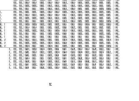
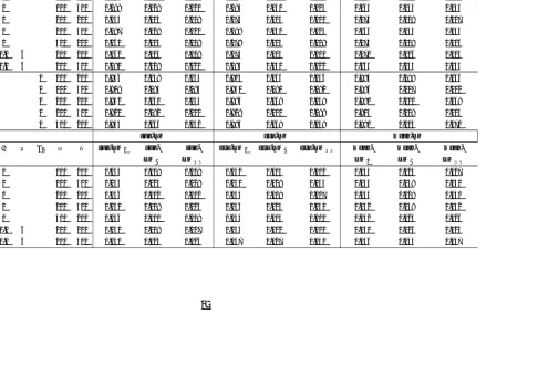
Table 1.1 size of Structural Break Tests with Known Break Date . . . 31

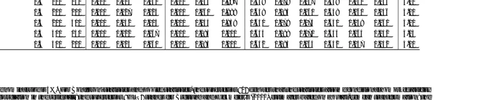
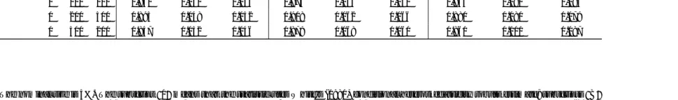
Table 1.2 Power against a Break at T /2 under DGP A1 . . . 33

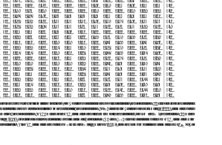
Table 1.3 Power against a Break at T /2 under DGP A2 . . . 34

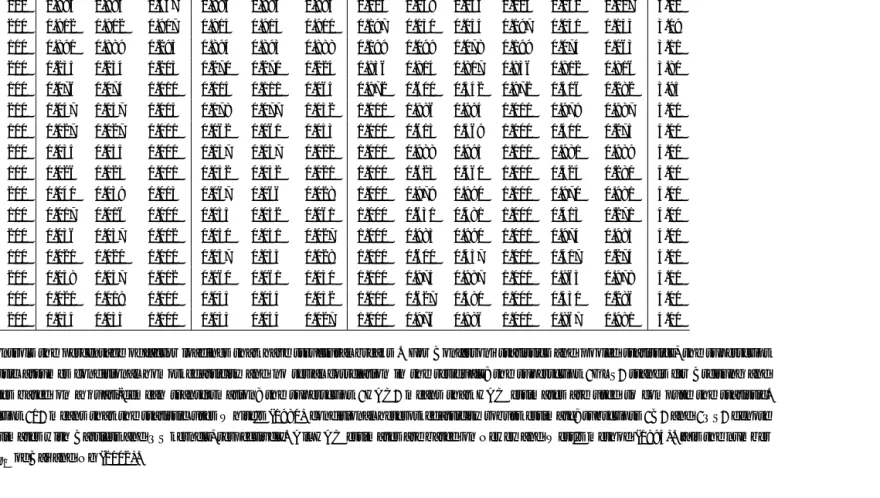
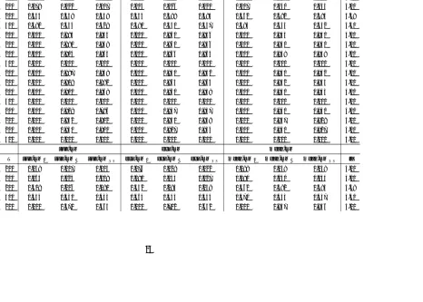
Table 1.4 Size of Structural Break Tests with Unknown Break Date . . . 35

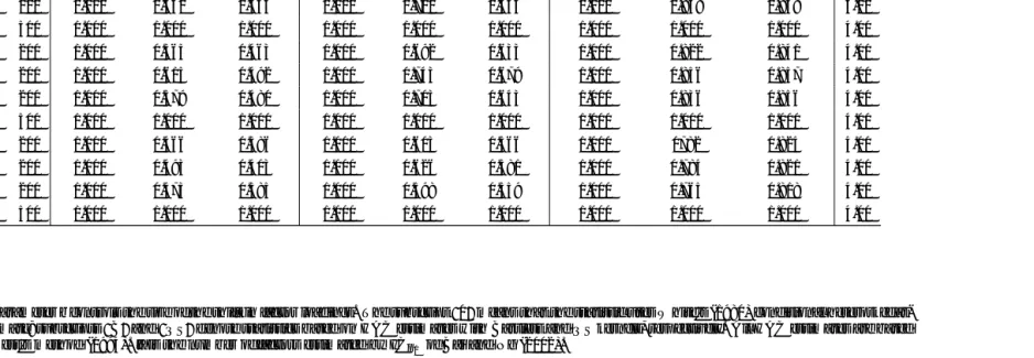
Table 1.5 Power against Unknown Break Date under DGP A1 . . . 37

Table 1.6 Power against Unknown Break Date under DGP A2 . . . 39

Table 1.7 Local Power with Known Break Date, N = 500, T = 500, r = 3 . . . 41

Table 1.8 Local Power with Unknown Break Date, N = 500, T = 500, r = 3 . . . 41

Table 1.9 Numbers of Factors in the Full Sample and Subsamples . . . 42

Table 1.10 Tests for Structural Breaks in Factor Loadings . . . 42

Table 1.11 Tests for Structural Breaks in Factor Dynamics . . . 44

Table 2.1 Means and modes of different estimators under DGP1 . . . 71

Table 2.2 Means and modes of different estimators under DGP2: subcase (1) . . . . 72

Table 2.3 Means and modes of different estimators under DGP2: subcase (2) . . . . 73

Table 2.4 Robustness of different estimators to the choice ofkmax . . . 74

Table 3.1 Size of Tests for the Overidentifying Restrictions under DGP N1 . . . 110

Table 3.2 Size of Tests for the Overidentifying Restrictions under DGP N2 . . . 111

Table 3.3 Power of Tests for the Overidentifying Restrictions under DGP A1 . . . 112

Table 3.4 Power of Tests for the Overidentifying Restrictions under DGP A2 . . . 113

(9)

LIST OF FIGURES

Figure 1.1 LMQS and WQS Statistics at different potential break points . . . 43

Figure 3.1 Impulse Responses of Macroeconomic Variables to a Unity Variance

Con-tractionary Monetary Policy Shock . . . 115

Figure 3.2 The Impulse Responses (in Percentage) of Price Indexes to a Unity

(10)

1 TESTS FOR PARAMETER INSTABILITY IN DYNAMIC

FACTOR MODELS

1.1 Introduction

Dynamic factor models have become popular in the recent macroeconometrics literature

be-cause a few factors can often explain a substantial amount of variations of many

macroeco-nomic time series. For example, they have been successfully used in forecasting (Stock and

Watson, 2002a), factor augmented vector autoregressive (FAVAR) models (Bernanke, Bivin

and Ellasz, 2005; Stock and Watson, 2005) and DSGE models (Boivin and Giannoni, 2006).

While most of these applications implicitly assume that the factor loadings in dynamic factor

models are time-invariant, there are strong evidence of structural instability in macroeconomic

time series (Stock and Watson, 1996). If the common factors are driven by some structural

shocks, it is possible that macroeconomic variables react to these structural shocks differently

during different sample periods, resulting in time-varying factor loadings. For example,

Eick-meier, Lemke and Marcellino (2011) consider time-varying FAVAR models to take into account

changes in the monetary transmission mechanism. In such cases, the dynamic factor models

may perform poorly or give misleading results. For example, Banerjee and Marcellino (2008)

provide simulation evidence that the performance of forecasts based on dynamic factor models

will be significantly worse off if the structural breaks in factor loading are ignored. While the

estimated factors still consistently span the original factor space if the size of breaks is local

to zero (Stock and Watson, 2002b), such results do not hold when the size of breaks is large.

Stock and Watson (2009) show that the coefficients on factors in a forecasting regression are

determined by factor loadings and the dynamic of factors, and their empirical results indicate

that factors estimated using the full sample can be still used in the forecast regression as long as

coefficients on the factors are allowed to be time-varying. In other words, the knowledge about

the existence of structural breaks of factor loadings and break dates are essential for forecasting

(11)

In this chapter, we consider testing the joint null hypothesis that factor loadings are constant

over time against the alternative that a non-negligible fraction of or all factor loadings are not.

We are interested in the joint null hypothesis rather than the null hypothesis that a specific

individual factor loading is constant over time because it is the joint null hypothesis under

which one can estimate the factors consistently. Conventional tests of structural change, such

as Andrews (1993), are designed to deal with finitely many parameters and cannot be used to

test our null hypothesis that involves parameters whose number goes to infinity as the sample

size grows. Directly extending the conventional test to our setup is challenging for two reasons.

First, one needs to estimate an infinite dimensional covariance matrix and its inverse. This

brings several technical difficulties: (1) the norm of the difference between the estimated and

true covariance matrices can be very large even if each entry of the estimated matrix converges

in probability; (2) taking the inverse of a high dimensional matrix will amplify the estimation

error dramatically and lead to very poor results (Ledoit and Wolf, 2004); and (3) the number

of time periods,T, can be even smaller than the dimension of the estimated covariance matrix,

so the covariance matrix can be singular. Second, because the degree of freedom also goes to

infinity, the limit distribution of such test statistics, even if it is well-defined, is likely to be

nonstandard.

To the best of our knowledge there are three existing tests for structural instability of factor

loadings. One is proposed by Stock and Watson (2009) (henceforth SW), who regressed each

variable on the estimated factors and implemented Chow-test for each of these regressions.

Using a post-war quarterly data set for the United States, they found a substantial amount of

instability in factor loadings: 41% (23%) of these Chow tests reject at the 5% (1%) significance

level. This method cannot control the overall type I error for testing our joint null hypothesis

and it may overstate the parameter instability in factor loadings. The other test is proposed

by Breitung and Eickmeier (2011) (henceforth BE). They constructed a joint test that controls

the overall type I error as well as tests for individual factor loadings allowing for an unknown

(12)

statistics for each of the factor loadings. They require that the idiosyncratic shocks be

cross-sectionally independent, however. This is more restrictive than Bai and Ng’s (2002) setup for

approximate factor models where idiosyncratic shocks are allowed to have weak cross-sectional

correlation. Also, their joint test is severely oversized in the presence of serial correlations in

the idiosyncratic shocks when the HAC covariance matrix estimator is used. 1

This chapter proposes new joint tests that circumvent these issues and contributes in the

following ways: First, we reduce the infinite-dimensional problem to a finite-dimensional one.

Because the principal component analysis implicitly imposes the restriction that the factor

loadings are time-invariant, the estimated factors will demonstrate a higher dimension under

the alternative hypothesis than under the null. Based on this fact, our statistic compares the

pre- and post-break subsample second moments of estimated factors. We allow for unknown

break dates and our statistic has the same asymptotic distribution as the conventional supreme

Wald test proposed by Andrews (1993). Second, we follow Bai and Ng’s (2002) approximate

factor setup in which serial, cross-sectional correlation and heteroskedascitity are allowed in the

idiosyncratic shocks, and the knowledge about the form of such correlations and

heteroskedas-ticity is not required to implement our test. This is more general than BE’s framework which

requires cross-sectional independence and AR(p) assumption on the idiosyncratic shocks. Third,

the number of factors are unknown and to be determined. To implement the test in this

chap-ter, the number of factors is estimated using the information criteria (IC) proposed by Bai and

Ng (2002). Both SW and BE point out that the number of factors will be enlarged when there

are structural breaks in factor loadings, BE remark that using IC to determine the number of

factors can reduce the power of each individual LM statistic. However, we show that Bai and

Ng’s IC remain consistent for estimating the enlarged dimension under the one-time break

al-1_{In the working paper version, they provide simulation evidence that the effective size of their test can be}

(13)

ternative and that this helps our test statistic to distinguish the null and alternative hypotheses,

i.e., it improves rather than reduces the power of our test. We find that if the estimated factors

are divided into pre- and post-break subsamples, then the sample second moments of estimated

factors in both subsamples will converge to the same limit under the null and different limits

under the alternative. Finally, we establish the regularity conditions on N, T and bandwidth

parameters for different kernel functions so that HAC estimators are applicable for our test

statistics. The technical details will be discussed in section 1.2.

In this chapter, all limits are taken as both N, T → ∞ simultaneously. ∥ · ∥ denotes the Euclidean norm of a vector or matrix, →p denotes convergence in probability, →d denotes convergence in distribution,⇒denotes weak convergence of stochastic processes, and⌊·⌋ is the integer part operator. Vech(·) is equal to the column-wise vectorization of a square matrix with the upper triangular excluded.

The remainder of this chapter is organized as follows: Section 1.2 proposes a structural

break test for factor loadings, and the asymptotic properties are established under the null and

alternative hypotheses. Section 1.3 shows Monte Carlo results under various data generating

processes (DGPs). Section 1.4 applies our tests to post-war quarterly macroeconomic time

series for the United States. We find some evidence that factor loadings changed in early 1980s.

Section 1.5 concludes. Proofs are relegated to appendices.

1.2 A Structural Break Test in Factor Loadings

1.2.1 Factor Models and the Null Hypothesis of Interest

Let xit denote the observation for the ith cross section and at period t for i= 1,2, ..., N and

t = 1,2, ..., T. Suppose that xit has r common factors and has the following static factor

representation:

xit =

    

f_t′λi1+eit fort = 1,2, ...,⌊πT⌋

f_t′λi2+eit fort = ⌊πT⌋+ 1,⌊πT⌋+ 2, ..., T

(14)

whereft is ar×1 vector of common factors at periodt,λi is ar×1 vector of factor loadings for the ith cross section, and eit is the idiosyncratic shock for cross section i at period t and

π∈(0,1). In the matrix notation

X =

   F1Λ

′

1

F2Λ′2

 

+e (1.2)

whereX = (X1, X2, ..., XN), Xi = (xi1, xi2, ..., xiT)′,F1 = (f1, f2, ..., f_⌊πT⌋))′,F2= (f_⌊πT⌋+1,

f_⌊_πT_⌋₊₂, ..., fT)′, Λj = (λ1j, λ2j, ..., λN j)′,e= (e1, e2, ..., eN), andei= (ei1, ei2, ..., eiT)′. We are interested in testing the null hypothesis of no break in the factor loadings:

H0 : λi1 =λi2for∀ (1.3)

The test of Breitung and Eickmeier (2011) is designed to test the null hypothesis

HBE,0: λi1 = λi2for giveni (1.4)

While their test is useful when one is interested in a specific factor loading, it is (1.3) under

which factors are consistently estimated. If their test for (1.4) is applied to test (1.3), the null

hypothesis (1.3) will be rejected with probability approaching one because the test is applied

to factor loadings whose number goes to infinity. Breitung and Eickmeier (2011) also suggest a

pooled LM test for testing (1.3) but their pooled test requires that the idiosyncratic shocks eit

are uncorrelated acrossi and thus rules out approximate factor structures. Below we propose

a test for the null hypothesis (1.3) that is valid under more general assumptions.

1.2.2 The Test Statistic

We consider a statistic that tests the null hypothesis H0: all factor loadings are constant over

time against the alternative hypothesis H1: αN many variables have structural changes in

(15)

our test statistic, consider a simple example. Under the null hypothesis note that (1.2) can be

rewritten in the following form:

X=

   F1

F2

  Λ′+e

where F1 is the pre-break subsample of F and F2 is the post-break subsample of F. If the

fourth moment offt is time-invariant, a Wald statistic comparingF₁′F1/⌊π∗T⌋andF2′F21/(T−

⌊π∗T⌋) should converge to a chi-square distributed random variable under the null hypothesis. Under the alternative hypothesis, (1.2) will have time-varying factor loadings, but conventional

principal component analysis (PCA) implicitly assumes that factor loadings are constant over

time. This means that we estimate an equivalent factor model with time-invariant factor

loadings:

X =

 

 F1 0⌊π∗T×r⌋

0_⌊(1−π∗)T×r⌋ F2

  Θ′+e

where Θ ≡[Λ1...Λ2], and Λ1 and Λ2 are pre- and post-break factor loadings, respectively. Let

G1 ≡[F1...0],G2 ≡[0...F2], andG≡[G′1...G′2]′. Note that

1 π∗TG

′

1G1 =

  

1

π∗TF1′F1 0r×r 0r_×r 0r×r

  

and

1 (1−π∗)TG

′

2G2 =

 

 0r×r 0r×r

0r×r ₍₁₋_π1∗₎_TF2′F2

  

have different limits, so the Wald test that compares the second moments ofG1 and G2 rejects

the null hypothesis under the alternative. This example shows that testing the structural

breaks in factor loadings is equivalent to testing the structural changes in the subsample second

moments of factors. Using this fact, we can reduce the indimensional problem to a

finite-dimensional one.

(16)

of ˆftfˆt′. Let A(π,Fˆ) ≡ vech

(_√

T

(

1

⌊πT⌋

∑_⌊πT⌋

t=1 fˆtfˆt′−T−⌊1πT⌋

∑T

t=⌊πT⌋+1fˆtfˆt′

))

. S(π,ˆ Fˆ) and

˜

S(π,F) denote unrestricted and restricted estimates of the long-run covariance matrix ofˆ

A(π,Fˆ), respectively, and will be defined more precisely in the next subsection. We define

two test statistics by

sup π∈[π1,π2]

WT(π,Fˆ) ≡ sup π∈[π1,π2]

A(π,Fˆ)′S(π,ˆ Fˆ)−1A(π,Fˆ), (1.5)

sup π∈[π1,π2]

LMT(π,Fˆ) ≡ sup π∈[π1,π2]

A(π,Fˆ)′S(π,˜ Fˆ)−1A(π,Fˆ), (1.6)

whereWT(π,F) andˆ LMT(π,Fˆ) are Wald and LM-like statistics for testing whether the

subsam-ple means of ˆftfˆt′ are equal or not at a predetermined break dateπT. The next two subsections will discuss the detailed properties of the proposed test statistics.

1.2.3 Asymptotics under the Null Hypothesis

We make the following assumptions under the null hypothesis.

Assumption 1: E∥ft∥4 < ∞, E(ftft′) = ΣF and T−1

∑_T

t=1ftft′ → ΣF as T → ∞ for some

positive definite matrix ΣF.

Assumption 2: ∥λi∥ ≤λ <¯ ∞, ∥Λ′Λ/N −ΣΛ∥ →0 for some r×r positive definite matrix ΣΛ,

and ∥Λ′Λ/N −ΣΛ∥ ≤O

(

1

√

N

)

.

Assumption 3: There exists a positive constantM <∞ such that for all N and T,

(a)E(eit) = 0,E|eit|8 ≤M for all iand t.

(b)E(e′_set/N) =E(N−1∑N_i₌₁eiseit) =γN(s, t),|γN(s, s)| ≤M for all s, andT−1∑T_s₌₁∑T_t₌₁

|γN(s, t)| ≤M.

(c)E(eitejt) =τij,twith|τij,t| ≤ |τij|for someτijand for all t. In addition,N−1∑N_i₌₁∑N_j₌₁|τij| ≤ M.

(d)E(eitejs) =τij,ts, and (N T)−1

∑_N

i=1

∑_N

j=1

∑_T

s=1

∑_T

t=1|τij,ts| ≤M. (e) for every (t, s),EN−1/2∑N_i₌₁[eiseit−E(eiseit)]

4

(17)

Assumption 4: E

(

1

N

∑_N

i=1√1_T

∑_T

t=1fteit 2)

≤M.

Assumption 5: There exists M < ∞ such that for all T and N, and for every t ≤ T and for

everyi≤N:

(a)∑T_s₌₁|γN(s, t)| ≤M. (b)∑N_k₌₁|τki| ≤M.

Assumption 6: There exists anM <∞ such that for all N and T:

(a) for each t, E_√1

N T

∑T s=1

∑N

k=1fs[eksekt−E(eksekt)]

2

≤M. (b)E√1

N T

∑T t=1

∑N

k=1ftλ′kekt≤M (c) for each t, E√1

N

∑_N

i=1λieit 4

≤M.

Assumption 7: The eigenvalues of r×r matrix (ΣΛΣF) are distinct.

Assumption 8: For any constantsπ1 and π2 that satisfy 0< π1 ≤π2 <1,

(a) sup_π_∈_[_π₁_,π_2]_√1

N T

∑_⌊πT⌋ t=1

∑N

k=1ftλ′kekt

2

=Op(1) and supπ∈[π1,π2]∥ 1

√

N T

∑T

t=⌊πT⌋+1

∑N k=1

ftλ′kekt∥2=Op(1). (b) sup_π_∈_[_π₁_,π_2] √T

⌊πT⌋

∑⌊πT⌋

t=1 (ftft′−ΣF)=Op(1) and supπ∈[π1,π2]∥

√

T T−⌊πT⌋

∑T

t=⌊πT⌋+1(ftft′− ΣF)∥=Op(1).

These assumptions are either from or slight modifications of those in Bai (2003). Assumption

1 is the same as Assumption A in Bai (2003) except that it requires that the second moment of

ft has to be constant over time. When there is a change in the stochastic process for factors,

this assumption is violated and our test may reject the null hypothesis even if factor loadings are

time-invariant. Given the results of Bai (2003), however, this assumption that there is no change

in the process of factors (e.g., autoregressive parameters and innovation variances) is testable

using conventional tests of structural change under our null hypothesis. The Assumption 2 is

different from Assumption B of Bai (2003) in that it specifies the convergence speed of Λ′Λ/N.2

2

(18)

Assumptions 3 - 5 and 7 exactly follow from Bai’s (2003) setup. Assumption 3 allows weak serial

and cross-sectional dependence in the idiosyncratic shocks, and Assumption 5 is a strengthened

version of Assumption 3. Assumptions 3 and 5 also allow heterogeneity in time and cross

section dimensions. Thus, this chapter allows weaker assumptions on idiosyncratic shocks than

BE who assume that the idiosyncratic shocks are cross-sectional independent and follow AR(p)

processes. Parts (a) and (b) of Assumption 6 are the same as Assumptions F1 and F2 of Bai

(2003). Assumption 6(c) is slightly stronger than the assumption of Bai (2003) which only

requires the second moment exists, but the asymptotic normal distribution of √1

N

∑N i=1λieit

and √1

T

∑T

t=1fteit in Bai (2003) is not necessary in this chapter. Assumption 8 states that the

terms in∥.∥areOp(1) uniformly inπ. Note that all summands have zero means, so Assumption 8 is an implication of the conventional functional central limit theorem.

Before discussing the properties of our test statistic, it is useful to describe some useful notations

and existing results. Let VN T be the r×r diagonal matrix of the first r largest eigenvalues of (1/T N)XX′ in decreasing order. Lemma A3 of Bai (2003) shows that VN T converges to V in probability, where V is the diagonal matrix consisting of the eigenvalues of Σ

1 2 ΛΣFΣ

1 2 Λ

in descending order. Let Υ denote Σ

1 2 ΛΣFΣ

1 2

Λ’s eigenvectors that corresponds to V such that

Υ′Υ =Ir. Recall that the estimated factor matrix ˆF is

√

T times eigenvectors corresponding to

the r largest eigenvalues ofXX′. LetH= (Λ′Λ/N)(F′F /T)Vˆ _{N T}−1 be anr×rmatrix. Proposition 1 of Bai (2003) show that F′F /Tˆ converges to Σ−

1 2

Λ ΥV

1

2. Thus, it follows thatH→p Σ 1 2 ΛΥV−

1 2.

LetH0 ≡plimT ,N→∞H , so it is obvious that

E(H₀′ftft′H0) =H0′ΣFH0=Ir (1.7)

which is implied by the definition ofH0and the fact thatV− 1 2Υ′Σ

1 2 ΛΣFΣ

1 2 ΛΥV−

1 2 =V−

1 2V V−

1 2 =

Ir.

Equation (1.7) provides a bridge connecting the statistics using estimated factors and true

factors. Let A(π, F H0) ≡ vech

(_√

T(_⌊_πT1 _⌋∑⌊_t₌₁πT⌋H₀′ftft′H0−_T_−⌊1_πT_⌋

∑_T

t=⌊πT⌋+1H0′ftft′H0

))

.

(19)

Under Assumption 1 that E(ftft′) = ΣF for∀t, the conventional central limit theorem implies thatA(π, F H0) converges in distribution to some normally distributed random variable. and a

Wald statistic or supreme Wald statistic can be constructed based onA(π, F H0) and its sample

variance. Although bothF and H0 are not observable, ˆF is a consistent estimate ofF H (see

Bai, 2003) and H→p H0, so replacingH0′ftby ˆft is a potential solution.

Theorem 1: Under Assumptions 1 - 8, if

√

T

N →0 asN, T → ∞, then

sup π∈[π1,π2]

A(π,Fˆ)−A(π, F H0)

p

→0

Theorem 1 shows that the difference between A(π,F) andˆ A(π, F H0) is op(1) uniformly in π,

so A(π,Fˆ) and A(π, F H0) will have the same asymptotic distribution. To construct a Wald

statistic, we also need the sample variance ofA(π, F H0). Let

Ω≡ lim T→∞Var

(

vech

(

1

√

T

( _T ∑

t=1

H₀′ftf_t′H0−Ir

)))

Let ˆΩ1(π, F H0) and ˆΩ2(π, F H0) be consistent estimates of Ω, where the subscript m = 1,2

denotes the pre- and post-break subsamples, respectively,π denotes the break date that splits

the sample, andF H0means that the sample variance is computed using unobservedft′H0. Since

the common factors ft are likely to be serially correlated, we consider the following estimates

for the sample variances:

ˆ

Ω1(π, F H0) =

⌊πT_∑⌋−1

j=0

k

(

j S_⌊πT⌋

)

ˆ

Γ1,j(π, F H0) +

⌊πT_∑⌋−1

j=1

k

(

j S_⌊πT⌋

)

ˆ

Γ1,j(π, F H0)′

ˆ

Ω2(π, F H0) =

T−⌊_∑πT⌋−1

j=0

k

(

j ST_−⌊πT_⌋

)

ˆ

Γ2,j(π, F H0) +

T−⌊_∑πT⌋−1

j=1

k

(

j ST_−⌊πT_⌋

)

ˆ

(20)

wherek(·) is a real-valued kernel

ˆ

Γ1,j(π, F H0) =

1

⌊πT⌋

⌊_∑πT⌋

t=j+1

vech(H₀′ftft′H0−Ir)vech(H0′ft−jft′−jH0−Ir)′

ˆ

Γ2,j(π, F H0) =

1 T − ⌊πT⌋

T

∑

t=j+⌊πT⌋+1

vech(H₀′ftft′H0−Ir)vech(H0′ft−jft′−jH0−Ir)′(1.9)

Alternatively, we can use all data to estimate ˆΩ1(π, F H0) and ˆΩ2(π, F H0),

ˆ

Ω(F H0) =

T_∑−1

j=0

k

(

j ST

)

ˆ

Γj(F H0) +

T_∑−1

j=1

k

(

j ST

)

ˆ

Γj(F H0)′ (1.10)

where

ˆ

Γj(F H0) =

1 T

T

∑

t=j+1

vech(H₀′ftft′H0−Ir)vech(H0′ft−jft′−jH0−Ir)′ (1.11)

In this paper, we focus our analysis on three commonly used kernels that always give positive

definite estimates: Bartlett, Parzen and Quadratic Spectral (henceforth QS).S is a band-width

parameter, and its subscript denotes the size of the sample (or subsample) that is used to

estimate the long-run variance. Let ˆS(π, F H0)≡ 1_πΩˆ1(π, F H0) +₁₋1_πΩˆ2(π, F H0), so ˆS(π, F H0)

is a consistent estimate of the asymptotic variance of A(π, F H0). One can also construct

the restricted estimate ˜S(π, F H0) using ˆΩ(F H0), i.e. ˜S(π, F H0) ≡ _π1Ω(F Hˆ 0) + ₁₋1_πΩ(F Hˆ 0).

Similar toA(π, F H0), ˆΩm(π, F H0), ˆΓm,j(π, F H0), form= 1,2, ˆΩ(F H0), ˆΓj(F H0), ˆS(π, F H0)

and ˜S(π, F H0) are computed using infeasible data ft′H0. We define ˆΩm(π,Fˆ), ˆΓm,j(π,Fˆ), for m = 1,2, ˆΩ( ˆF), ˆΓj( ˆF), ˆS(π,Fˆ) and ˜S(π,Fˆ) as the feasible analogs computed using the

estimated regressors ˆF.

Condition 1: (a) The Bartlett kernel is used to estimate ˆS(π, F H0), ˆS(π,F), ˜ˆ S(π, F H0) and

˜

S(π,F), and there exists a constantˆ K > 0 such that ST, S⌊πT⌋, and ST−⌊πT⌋ are less than KT13 for all π∈[π₁, π₂]⊂(0,1); and (b) T

2 3

N →0 as N, T → ∞.

(21)

˜

S(π,F), and there exists a constantˆ K >0 such thatST,S_⌊πT⌋, andST−⌊πT⌋are less thanKT

1 5

for allπ ∈[π1, π2]⊂(0,1); or, the QS kernel is used to estimate ˆS(π, F H0), ˆS(π,Fˆ), ˜S(π, F H0)

and ˜S(π,F), and there exists constantsˆ K1, K2 >0 such thatK1T 1

5 ≤ST, S_⌊_πT_⌋, S_T_−⌊_πT_⌋≤

K2T 1

5 for all π∈[π₁, π₂]⊂(0,1); and (b) T 2 5

N →0 as N, T → ∞.

Theorem 2: Under Assumptions 1 - 7, if Condition 1 or Condition 2 holds, then

sup π∈[π1,π2]

_S(π,ˆ _Fˆ₎₋_{S(π, F H}ˆ ₀₎_→p ₀

and

sup π∈[π1,π2]

_S(π,˜ _Fˆ₎₋_{S(π, F H}˜ ₀₎ p

→0

Theorem 2 shows that the infeasible sample variance can be replaced by the estimates computed

using ˆF. Given this result, we can compute the Wald statisticWT(π,Fˆ)≡A(π,Fˆ)′Sˆ−1A(π,Fˆ), the LM-like statistic LMT(π,Fˆ)≡A(π,Fˆ)′S˜−1A(π,Fˆ), supWT(π,Fˆ) and supLMT(π,Fˆ). To establish the asymptotic distributions for these statistics, we make the following assumption:

Assumption 9: (a) Ω ≡ limT→∞Var

(

vech

(

1

√

T

(∑T

t=1H0′ftft′H0−Ir

)))

is positive definite,

and ∥Ω∥<∞. Let ˆΩ1(π, F H0) and ˆΩ2(π, F H0) be consistent estimators of Ω satisfying that

sup π∈[π1,π2]

_{Ωm(π, F H}ˆ ₀₎₋_Ω₌_{op(1) for} _m_{= 1,}₂

(b)WT(π, F H0)≡A(π, F H0)′S(π, F Hˆ 0)−1A(π, F H0)⇒ Qp(π) and supπ∈[π1,π2]WT(π, F H0)

d

→

sup_π_∈_[_π₁_,π_2]Qp(π), where Qp(π) = [Bp(π)−πBp(1)]′[Bp(π)−πBp(1)]/[π(1−π)] andBp(·) is a p-vector (p= r(r₂+1)) of independent Brownian motions on [0, 1] restricted to [π1, π2]⊂(0,1).

Assumption 9(a) states that ˆΩm(π, F H0) converges to the population moment Ω uniformly

inπ. This is similar to Assumption 3 of Andrews (1993). Assumption 9(b) is just the main result

(22)

to the stochastic process Qp(π) restricted to [π1, π2] ⊂ (0,1), and supπ∈[π1,π2]WT(π, F H0)

converges to sup_π_∈_[_π₁_,π_2]Qp(π) by the continuous mapping theorem. Note that all the terms in Assumption 9 are computed using the infeasible data F H0, which means that if F H0 were

observable, one would be able to use the conventional supreme Wald test. The following theorem

guarantees that one can use the estimated regressors, ˆF, to compute the sup-W statistic, which

has the same asymptotic distribution as the one computed usingF H0.

Theorem 3: Under Assumptions 1 – 9, if either Condition 1 or Condition 2 holds and

√

T N →0 asN, T → ∞, then

(i) sup_π_∈_[_π₁_,π₂_]WT(π,Fˆ)−WT(π, F H0)=op(1) and supπ∈[π1,π2]

LMT(π,F)ˆ −LMT(π, F H0)

=op(1).

(ii) sup_π_∈_[_π₁_,π_2]WT(π,Fˆ) d

→sup_π_∈_[_π₁_,π_2]Qp(π) and supπ∈[π1,π2]LMT(π,Fˆ)

d

→sup_π_∈_[_π₁_,π_2]Qp(π).

Theorem 3 shows that one can use the conventional critical values for the sup-W and

sup-LM statistic computed using ˆF. The uniformity provided by part (i) of Theorem 3 also

shows that WT(π,F)ˆ ⇒ Qp(π) and LMT(π,Fˆ) ⇒ Qp(π) by assumption 9(b). Thus, the continuous mapping theorem implies that the mean Wald statistic and the average exponential

Wald statistic proposed by Andrews and Ploberger (1994) can also be used to test structural

breaks in factor loadings.

Corollary 1: Under Assumptions 1 – 9, if Condition 1 or Condition 2 holds and

√

T

N → 0 as N, T → ∞, then

ˆ π2

π1

exp

(

WT(π,Fˆ) 2

)

dπ− ˆ π2

π1

exp

(

WT(π, F H0)

2

)

dπ=op(1)

ˆ π2

π1

WT(π,F)dπˆ − ˆ π2

π1

WT(π, F H0)dπ=op(1)

Define exp-W( ˆF)≡ln

(

1

π2−π1 ´π2

π1 exp

(

WT(π,Fˆ) 2

)

dπ

)

and mean-W( ˆF)≡ _π 1

2−π1 ´π2

π1 WT(π,

ˆ F)dπ.

Corollary 1 shows that critical values provided by Andrews and Ploberger (1994) can be

(23)

also holds for exp-LM( ˆF) and mean-LM( ˆF) which can be defined in a similar way.

1.2.4 Asymptotics under the Alternative Hypothesis

We consider the alternative hypothesis that a fraction of or all factor loadings have a single

break at a common break date. Let ⌊π∗T⌋+ 1 denote the break date of factor loadings. The factor F = (f1, f2, ..., fT)′ is aT×r matrix. ft can be written as ft= (f0′,t, f1′,t)′, wheref0,t is a q0×1 vector that denotes the factors that have time-invariant factor loadings, f1,t is a q1×1

vector that denotes the factors whose loadings change at⌊π∗T⌋+ 1, andr=q0+q1. The factor

model can be written as:

Xit =

      

f₀′_,tλ0,i+f1′,tλ1,i+eit if 1≤t≤ ⌊π∗T⌋ f₀′_,tλ0,i+f1′,tλ2,i+eit if ⌊π∗T⌋+ 1≤t≤T

(1.12)

where λ0,i is the factor loading of f0,t, and λ1,i and λ2,i are the pre- and post-break factor

loadings off1,t, respectively. The model can be also expressed in a matrix form:

X=

 

 F0,1 F1,1 0

F0,2 0 F1,2

         

Λ′₀ Λ′₁ Λ′₂

      

+e (1.13)

whereF0,1 = (f0,1, f0,2, ..., f0,⌊π∗T⌋)′,F0,2= (f0,⌊π∗T⌋+1, f0,⌊π∗T⌋+2, ..., f0,T)′,F1,1 = (f1,1, f1,2, ...,

f₁_,_⌊_π∗_T_⌋)′,F2 = (f1,⌊π∗T⌋+1, f1,⌊πT⌋+2, ..., f1,T)′, Λ0 = (λ0,1, λ0,2, ..., λ0,N)′, Λ1 = (λ1,1, ..., λ1,N)′, and Λ2 = (λ2,1, ..., λ2,N)′. Notice that Equation (1.13) is equivalent to a factor model that has r+q1 factors with time-invariant factor loadings, i.e.

(24)

where G =

 

 F0,1 F1,1 0

F0,2 0 F1,2

 

 is a T ×(r +q1) factor matrix, and Θ = [Λ0...Λ1...Λ2] is a

N×(r+q1) factor loading matrix. Letgtdenote thetthcolumn ofG′, i.e. gt≡(f0′,t, f1′,t,01×q1)′

if 1≤t≤ ⌊π∗T⌋, and gt≡(f0′,t,01×q1, f1′,t)′ if ⌊π∗T⌋+ 1≤t≤T. Let θi ≡(λ′0,i, λ′1,i, λ′2,i)′ so that Θ = (θ1, θ2, ..., θN)′. Let G1 ≡[F0,1...F1,1...0] and G2 ≡ [F0,2...0...F1,2]. Let ˆG, ˆG1, ˆG2 and ˆgt

denote the PCA estimates ofG,G1,G2 and gt.

To analyze the property of the test statistics under the alternative hypothesis, we make the

following assumptions:

Assumption 1’: maxt=1,...,T E∥gt∥4 <∞, T−1F0′,1F0,1

p

→ π∗Σ0,0,T−1F0′,2F0,2

p

→ (1−π∗)Σ0,0,

T−1F₀′_,₁F1,1

p

→ π∗Σ0,1, T−1F0′,2F1,2

p

→ (1−π∗)Σ0,2, T−1F1′,1F1,1

p

→ π∗Σ1,1, T−1F1′,2F1,2

p

→

(1−π∗)Σ2,2 and T−1G′G

p

→ΣGasT → ∞, where Σ0,0, Σ1,1, Σ2,2 and ΣG are positive definite. Assumption 2’: ∥θi∥ ≤θ <¯ ∞,∥Θ′Θ/N−ΣΘ∥ →0 for some (r+q1)×(r+q1) positive definite

matrix ΣΘ, and∥Θ′Θ/N −ΣΘ∥ ≤O

(

1

√

N

)

.

Assumption 3’: The same as Assumption 3.

Assumption 4’: E

(

1

N

∑_N

i=1√1_T

∑_T

t=1gteit 2)

≤M.

Assumption 5’: The same as Assumption 5.

Assumption 6’: There exists an M <∞ such that for all N and T:

(a) for each t, E√1 N T

∑_T

s=1

∑_N

k=1gs[eksekt−E(eksekt)] 2

≤M. (b)E_√1

N T

∑_T

t=1

∑_N

k=1gtθ′kekt≤M (c) for each t, E_√1

N

∑_N

i=1θieit

4

≤M.

Assumption 7’: The eigenvalues of (r+q1)×(r+q1) matrix (ΣΘΣG) are distinct.

Assumption 8’: For any constants π1 and π2 that satisfy 0< π1 ≤π∗ ≤π2<1, supπ∈[π1,π2]

1

√

N T

∑⌊t=1πT⌋

∑_N

k=1gtθk′ekt

=Op(1) and sup_π_∈_[_π₁_,π_2]√1

N T

∑T

t=⌊πT⌋+1

∑_N

k=1gtθ′kekt

(25)

Remarks: (1) The first part of Assumption 1’ that maxt=1,...,TE∥gt∥4 < ∞ is implied by

Assumption 1 that E∥ft∥4 < ∞, since gt ≡ (f0′,t, f1′,t,01×q1)′ if 1 ≤ t ≤ ⌊π∗T⌋, and gt ≡

(f₀′_,t,01×q1, f1′,t)′ if⌊π∗T⌋+ 1≤t≤T. However, E(gtg′t) is not constant over time. Also, Σ1,1

and Σ2.2 can be different. This is different from Assumption 8(b) where two subsample averages

converge to the same limit. Thus, time-varyingE(gtg′_t) leads to Assumption 8’ only consisting of the analog of Assumption 8(a). Assumption 2’ allows thatλ1,i =λ2,i for somei, i.e. only a

fraction of factor loadings have structural breaks. The positive definiteness of ΣΘ rules out the

case where only o(N) many factor loadings are time-varying.

(2) Assumptions 2’ – 7’ are just analogs of Assumptions 2 – 7,3 and the difference is that the

factor ft is replaced bygt and the dimension of factor loadings is augmented from r tor+q1.

Thus, although Assumptions 1’ – 7’ look different from Assumptions 1 – 7, they still maintain

the canonical assumptions for (1.14) under the alternative hypothesis, and hence many results

in Bai and Ng (2002) and Bai (2003) are directly applicable.

We next define the analogs of VN T, V, Υ, H, and H0 under the alternative hypothesis.

Let UN T be the (r +q1)×(r+q1) diagonal matrix of the first r+q1 largest eigenvalues of

(1/T N)XX′in descending order. LetU be the probability limit ofUN T, whereUis the diagonal matrix consisting of the eigenvalues of Σ

1 2 ΘΣGΣ

1 2

Θ in descending order (Lemma A3, Bai and Ng,

2003). Let Ξ denote Σ

1 2 ΘΣGΣ

1 2

Θ’s eigenvectors that correspond toU such that Ξ′Ξ =Ir+q1. Let

J = (Θ′Θ/N)(G′G/Tˆ )U_{N T}−1 be an (r+q1)×(r+q1) matrix. Denote plimT ,N→∞J asJ0, which

is a non-singular matrix (see Proposition 1 of Bai, 2003). Finally, let

D1≡

      

Σ0,0 Σ0,1 0

Σ′₀_,₁ Σ1,1 0

0 0 0

      

, D2 ≡

      

Σ0,0 0 Σ0,2

0 0 0

Σ′₀_,₂ 0 Σ2,2

      

and C≡J₀′(D1−D2)J0. 3

(26)

To establish the consistency of the test under the alternative hypothesis, we need

Assump-tion 9’ that regulates the asymptotic property of the variance matrix in our statistics. Define

ˆ

Ω1(π∗, GJ0), ˆΩ2(π∗, GJ0), ˆΩ(GJ0) by replacing π,F,H0 andIrin equations 1.8, 1.9, 1.10, and

1.11 withπ∗,G,J0andIr+q1, respectively. Let ˆS(π∗, GJ0) = 1

π∗Ωˆ1(π∗, GJ0) +

1

1−π∗Ωˆ2(π∗, GJ0) and ˜S(π∗, GJ0) = _π1∗Ω(GJˆ 0) + ₁₋1_π∗Ω(GJˆ 0). Define ˆS(π∗,G) and ˜ˆ S(π∗,G) by replacingˆ GJ0

with ˆG.

Assumption 9’: (a)

plim_T_→∞inf

{

vech(C)′

[

max(S_⌊_π∗_T_⌋, S_T_−⌊_π∗_T_⌋) ˆS(π∗, GJ0)−1

]

vech(C)

}

>0

plim_T_→∞inf

{

vech(C)′

[

STS(π˜ ∗, GJ0)−1

]

vech(C)

}

>0

where S_⌊_π∗_T_⌋,S_T_−⌊_π∗_T_⌋, and ST are the bandwidth parameters for ˆΩ1(π∗, GJ0), ˆΩ2(π∗, GJ0),

and ˆΩ(GJ0), respectively.

(b) Condition 1 or 2 holds for ˆS(π∗, GJ0), ˆS(π∗,G), ˜ˆ S(π∗, GJ0), and ˜S(π∗,G).ˆ

Remark: Assumption 9’(a) ensures that WT(π∗, GJ0) and LMT(π∗, GJ0) diverge under the

alternative asT goes to infinity. Contrast to Equation 1.7, it is worth noting thatE(J₀′gtg′tJ0)̸=

Ir+q1 under the alternative hypothesis, so the HAC estimates are not properly demeaned. Hall

(2000) investigates the properties of HAC estimates that are not properly demeaned in the

context of overidentifying restriction tests. He shows that if the HAC estimate is not correctly

demeaned, then it will diverge at the rate of the bandwidth parameter BT. Theorem 2 of

Hall (2000) also shows that the overidentifying restrictions test statisticQT will diverge at the

rate T /BT and that (BTQT)/T is bounded away from zero as T goes to infinity. Although

Hall’s (2000) results are developed in the context of overidentifying restriction tests, they can

be readily extended to our test statistics, because these two types of statistics are constructed

using the same quadratic form. Assumption 9’(a) can be verified using Hall’s proof (2000,

(27)

Theorem 4: Under Assumptions 1’ – 9’,

(i) There exist some non-random matrixC̸= 0, such that _⌊_π_∗1_T_⌋∑_t⌊₌₁π∗T⌋gˆtgˆt′−_⌊T−1π∗T⌋

∑_T

t=⌊π∗T⌋+1

ˆ gtgˆt′

p

→C.

(ii) Suppose that vech(C) is not in the null space of [plim_N,T_→∞S(πˆ ∗,G)]ˆ −1and of [plim_N,T_→∞ ˜

S(π∗,G)]ˆ −1For any constantsπ1andπ2that satisfy 0< π1≤π∗ ≤π2<1, supπ∈[π1,π2]WT(π,G)ˆ

and sup_π_∈_[_π₁_,π_2]LMT(π,G) are consistent under the alternative hypothesis that a fraction ofˆ N cross sections have structural breaks in their factor loadings at a common time⌊π∗T⌋.

Remarks: (1) Theorem 4(i) shows that pre- and post-break subsample means of ˆgtgˆt′

con-verge to different limits under the alternative hypothesis. This explains why just using a Wald

statistic computed using estimated factors can in fact test the structural breaks in factor

load-ings. Note that the factors (in static form) are estimated by PCA which implicitly assumes

that the factor loadings are time-invariant. This implies that if there are structural breaks in

the factor loadings, then PCA will in fact estimate an equivalent factor model (see equation

(1.13)) with more factors and time-invariant factor loadings. Although both ˆF′F /Tˆ and ˆG′G/Tˆ are equal to identity matrices under the null and the alternative hypotheses, _⌊_πT1 _⌋∑_t⌊₌₁πT⌋fˆtfˆt′ and _T_−⌊1_πT_⌋∑T_t₌_⌊_πT_⌋₊₁fˆtfˆt′ converge to the same limit for any π ∈ [π1, π2] ⊂ (0,1), while

1

⌊π∗T⌋

∑⌊π∗T⌋

t=1 ˆgtˆg′tand _⌊T−1π∗T⌋

∑T

t=⌊π∗T⌋+1gtˆˆgt′ converge to different limits due to the augmented factor space caused by the implicit restriction of PCA that the factor loadings have to be

un-changed over time. Thus, distinguishing the null and the alternative hypotheses is equivalent

to comparing the pre- and post-break subsample means of ˆftfˆ_t′ or ˆgtˆg′_t.

(2) Note that different behaviors of ˆftfˆt′ and ˆgtˆgt′ result from the fact that both ˆG1 and ˆG2 do

not have full column ranks under the alternative hypothesis. This indicates that the number

of factors plays an important role in determining the asymptotics of the test statistics in this

paper. In practice, the number of factors is commonly estimated using IC proposed by Bai and

Ng (2002), so the asymptotics of IC under the null and alternative hypotheses will substantially

(28)

and Ng’s IC in fact help our statistics distinguish the null and alternative hypotheses in large

samples:

Proposition: Under Assumptions 1’–4’, Bai and Ng’s information criteria consistently

esti-mate the number of factors of the equivalent model (Equation 1.14).

What IC does is equivalent to determining the number of (asymptotically) non-zero eigenvalues

of XX′/N T. Under the null hypothesis, Assumptions 1 – 4 are just all assumptions that are required by Bai and Ng’s IC, so the number of factors, i.e. the number of non-zero eigenvalues of

XX′/N T, can be consistently estimated. Under the alternative hypothesis, Assumptions 1’ – 4’ are just the all assumptions required for the equivalent model with time-invariant factor loadings

(see Equation (1.13)), so IC will consistently estimate the number of factors r+q1. Thus, the

asymptotics of test statistics proposed in this paper will not be affected by implementing IC in

the first stage as N andT tend to infinity, and the finite-sample effect of the first-stage IC will

be investigated in Monte Carlo experiments in the next section.

(3) When IC is used in the first stage to determine the number of factors, tests for structural

breaks should not be based on the factor loadings. For example, the traditional Chow test for

testingλi1 =λi2 will not have power under the alternative hypothesis, because the factor

load-ings of the equivalent model,θi, are actually time-invariant under the alternative.4 Therefore,

in order to test structural breaks in factor loadings, one should focus on the estimated factors

rather than the estimated factor loadings.

1.3 Monte Carlo Simulations

In the Monte Carlo experiments we investigate the finite sample properties of our statistics for

known and unknown break points. Section 1.3.1 compares the performance of our Wald testW

and LM-like testLM with BE’s pooled testSBEand the Bonferroni testsBon, whereW andLM

4_{Breitung and Eickmeier (2011) also point out that the Chow test statistic will be lack of power if the number}

(29)

abbreviateWT(π,F) andˆ LMT(π,Fˆ),respectively. Recall thatSBE =

(∑N

i=1si−rN

)

/√2rN, where si is the LM statistic5 for the ith variable and r is estimated by Bai and Ng’s IC, ICp1

and ICp2. We use three different superscripts to denote the way to compute si: s 0

i denotes the

LM statistic assuming that the idiosyncratic shocks are conditional homoskedastic and serially

uncorrelated; sGLS_i denotes the LM statistic computed using quasi-demeaned residuals which

are based on AR models with lags selected by BIC; sHAC_i denotes the LM statistic computed

using HAC estimate. Let S0

BE,SBEGLS and SBEHAC denote the pool statistics computed using s0i,

sGLS_i and sHAC_i , respectively. Besides the pooled statistics, we also include the results based

on Bonferroni critical values: F−1(1−5%/N), where F is the chi-square CDF with degree of freedom ˆr. The reason for considering the Bonferroni test is that there are N individual LM

statistics si, using the 5% significance level for each si will always result in a fraction of all

si rejecting the null hypothesis even if the factor loading matrix is constant over time. The

Bonferroni method is a simple way to control the overall type I error of allsistatistics. Lets0_Bon,

sGLS_Bon and sHAC_Bon denote the Bonferroni statistics based on s_i0,sGLS_i and sHAC_i , respectively. In

addition, theW andLM statistics are computed using three different estimates for the sample

variances: W0 and LM0 are computed using White’s (1980) conditional heteroskedasticity

robust estimate; WB and LMB are computed using Newey and West’s (1994) data dependent

HAC estimate based on the Bartlett kernel;WQS andLMQS are computed using the same data

dependent HAC estimate but based on the QS kernel.

Section 1.3.2 compares the performance of the sup-W, exp-W, mean-W, sup-LM, exp-LM,

and mean-LM tests when a break date is unknown. Similar to Section 1.3.1, the subscripts “0”,

“B” and “QS” denote the statistics using the conditional heteroskedasticity robust estimate,

HAC estimate based on the Bartlett kernel, and HAC estimate based on the QS kernel,

respec-tively. Section 1.3.3 provides Monte Carlo experiments on the power comparison between our

and CDG’s tests.

In all Monte Carlo experiments, the R2 = trace(ee′)/trace(XX′) is set to be 50% and the

5

(30)

number of replications is 5000 for each DGP.

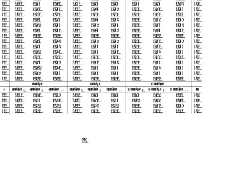
1.3.1 Testing Breaks with Known Break Date

Our first experiment focuses on the sizes of W, LM, sBon and SBE when the break date is

known. The model is xit =

∑r

k=1λikfkt+κeit, where λik ∼ i.i.d.N(b₂,1), and fkt and eit are generated by the following DGPs:

N1: fkt, eit∼i.i.d.N(0,1),κ=

√

(1 +b2_/4)r.

N2: fkt∼i.i.d.N(0,1),eit=σi(νit+

∑

1≤|j|≤Pβνi−j,t),σi ∼i.i.d.U(0.5,1.5), νit∼i.i.d.N(0,1), and κ=√12(1 +b2_{/4)r/13(1 + 2P β}2_).

N3: fkt = ρffkt₋1 +µit, µit ∼ i.i.d.N(0,1 −ρ2f), eit = σiνit, σi ∼ i.i.d.U(0.5,1.5), νit = ρννit−1+ϵit+ωϵϵit−1,ϵit∼i.i.d.N

(

0,₁₊₍_ρ 1

e+ωϵ)2/(1−ρ2e)

)

, and κ=√12(1 +b2_/4)r/13.

We setb= 1 in N1 – N3. N1 is the simplest DGP: both factors and idiosyncratic shocks are

i.i.d, i.e. no correlation or heteroskedasticity is involved. Both N2 and N3 allow

heteroskedas-ticity acrossi, and we follow Breitung and Eickmeier’s (2011) setup: σi ∼i.i.d.U(0.5,1.5). N2 also allows limited cross-sectional correlation in idiosyncratic shocks ifβ̸= 0 andP ≥1. We let β ∈ {0,0.1}and P ∈ {6,8}, and these values are similar to those of Onatski (2010). DGP N3 considers the the case where both factors and idiosyncratic shocks are serially correlated. The

factors are assumed to be AR(1) processes, and ρf = 0.7 which leads to mild persistency. νit

follows an AR(1) process ifωϵis zero, or an ARMA(1, 1) process otherwise. We setωϵ ∈ {0,0.5} and ρν = 0.5. Table 1.1 reports the the size of the Bonferroni test, BE’s pooled tests and our

tests. The last column of Table 1.1 is averaged number of factors selected byICp1 of Bai and

Ng (2002). Under DGPs N1 and N2 without cross-sectional correlation (β = 0), the sizes of

S_BE0 , S_BEGLS, W0 and LM0 are close to 5%. The tests based on the Bonferroni critical values

or HAC estimates are relatively conservative, but their rejection rates approach 5% as N and

T increase. Under DGP N2 with cross-sectional correlations (β ̸= 0 and P > 0), the pooled tests tend to over-reject the null hypothesis. For example, the effective size of S_BEGLS is 16.2%

(31)

arbitrary correlation across si, the size of s0Bon, sGLSBon and sHACBon does not exceed the nominal

level. Our tests are computed using ˆF which does not require the independence of idiosyncratic

shocks, so the size of our tests is robust to cross-sectional correlation in eit. The IC tends to

over-estimate the number of factors when the correlation is relatively strong. For instance,

when P = 8, β = 0.1, N = 100, and T = 200, the average of estimated number of factors is

6.37, but our test statistics are robust to this uncertainty caused by IC. Under DGP N3, SHAC BE

always rejects more than 75% of the times, which is similar to the results in the working paper

version of Breitung and Eickmeier (2011). The size ofS_BEGLS is close to 5% except in the cases

where N is relatively larger than T. The size of W and LM based on HAC estimates are not

far from 5%, andLM tends to have better size thanW for small T.

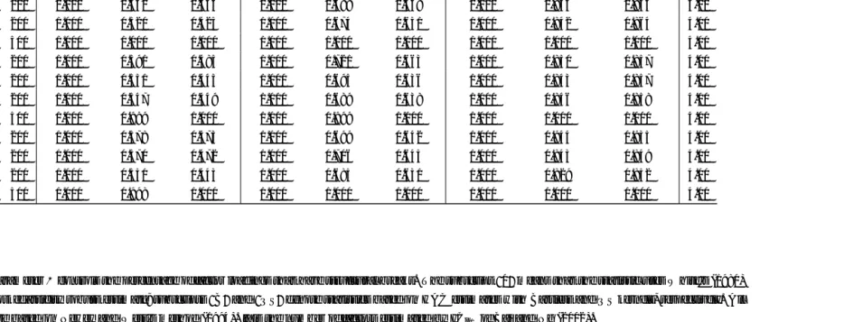
The second experiment compares the powers ofW,LM,sBonandSBE when the break date

is known. The break date is set to be T₂, and the data are generated by the following DGPs6:

A1: xit=∑r_k₌₁λikfkt+κeit for i= 1,2, ..., N and t≤T /2, and xit=∑r_k₌₁(λik−b)fkt+κeit for i = 1,2, ..., N and t ≥ T /2 + 1, where fkt, eit ∼ i.i.d.N(0,1), κ = √(1 +b2_{/4)r, and}

λik∼i.i.d.N(₂b,1). A2: xit =

∑_r

k=1λikfkt+κeit for i = 1,2, ..., αN and t ≤ T /2, xit =

∑_r

k=1(λik −b)fkt+τ eit for i = 1,2, ..., αN and t ≥ T /2 + 1, and xit =

∑r

k=1λikfkt+κeit for i= αN + 1, ..., N and

t= 1,2, ..., T, where fkt, eit ∼i.i.d.N(0,1), κ=

√

(1 +b2_/4)r,_λ

ik∼i.i.d.N(b₂,1), andb= 1. DGP A1 focuses on how the power changes as the magnitude of break in factor loadings

increases. We setb∈ {1/3, 2/3, 1, 2}. Table 1.2 summarizes the results under DGP A1. The power of the pooled tests and our tests have exactly the opposite pattern. When b= 1/3 and

N and T are relatively small, the pooled tests are very powerful, while ours do not have good

power. However, as N and T increase, our tests become powerful. When N and T = 500,

our test always reject the null, whereas the pooled tests reject less than 10%. Additionally,

when b becomes larger, LM and W are powerful even for small N and T, while the power of

the pooled tests is in fact close to the nominal size. The reason for this phenomenon is that

6

Structural Breaks, Model Selection, and Overidentification in Dynamic Factor Models.

ABSTRACT

BIOGRAPHY

TABLE OF CONTENTS

LIST OF TABLES

LIST OF FIGURES

1

TESTS FOR PARAMETER INSTABILITY IN DYNAMIC

FACTOR MODELS