Scheduling Precedence-Constrained Jobs On Two Resources To Minimize The Total Weighted Completion Time.

(1)

ABSTRACT

RAJNEESH, RAJNEESH. Scheduling Precedence-Constrained Jobs on Two Resources to Minimize the Total Weighted Completion Time. (Under the direction of Salah E. Elmaghraby.)

We study a problem of scheduling precedence-constrained jobs on two pre-specified

resources with the objective of minimizing the weighted completion time. We present

two mathematical formulations of the problem: a dynamic programming (DP) model

and a binary integer programming (BIP) model. Due to the strong N P-hardness of the problem, even for two resources with chain-type precedence constraints among the jobs

with weight and processing times of 1, we restrict our analysis to the case when the

precedence constraints result in a series-parallel (s/p) graph. We focus on reducing the

state space in the DP model to obtain an optimal, or near optimal, solution. We compare,

through a number of experiments with varying number of jobs, resource requirements,

and topology of the precedence among the jobs, the performance of the DP and the BIP

(2)

(3)

Scheduling Precedence-Constrained Jobs on Two Resources to Minimize the Total Weighted Completion Time

by

Rajneesh Rajneesh

A thesis submitted to the Graduate Faculty of North Carolina State University

in partial fulfillment of the requirements for the degree of

Master of Science

Operations Research

Raleigh, North Carolina

2012

APPROVED BY:

Yahya Fathi Matthias F. Stallmann

(4)

DEDICATION

(5)

BIOGRAPHY

Rajneesh was born in Ranchi, India. He attended Ranchi University, India and graduated

in 2002 with a Bachelor of Science in Mathematics as an honors subject. He continued

his studies further for Master of Science (M.Sc.) in Mathematics and Computing from

Indian School of Mines (ISM), Dhanbad, India and received M.Sc. degree in 2004.

After graduating from ISM, he received the opportunity to work in a sponsored

re-search from the Department of Science and Technology, India, to study the seismic

activ-ities in Eastern India. In 2005, he accepted an offer as a teaching assistant at the Indian

Institute of Management, Ahmedabad (IIMA). He received a Junior Research Fellowship

in 2006 from the Indian Space Research Organization (ISRO) and worked on the

numer-ical weather forecasting models. He accepted a position at the Indian School of Business

(ISB), Hyderabad in 2007 to work on a research project and as a teaching assistant.

He joined North Carolina State University in 2008 to pursue graduate studies in

Operations Research. He taught undergraduate Mathematics courses in the Fall of 2008

and the Spring of 2009. He was teaching assistant for graduate level OR courses during

the Fall of 2009, the Spring of 2010 and the Spring of 2011 semesters. He received a

full-time internship at the JMP development group at SAS Institute Inc., Cary, in the

Summer of 2010 and the Fall of 2010 semesters. He continued to work part-time at SAS

(6)

ACKNOWLEDGEMENTS

Foremost, I would like to thank my advisor, Dr. Salah E. Elmaghraby, who made this

work possible by introducing me to the research problem. I greatly appreciate his kind

and wise guidance throughout my research. Dr. Elmaghraby’s Dynamic Programming

(DP) class stimulated my interest in DP modeling approach and was very helpful in my

research formulation. I am particularly grateful to him for the patience he showed in me,

teaching me how to become a good researcher and a better person in life. Working with

him has been my best learning experience at NCSU and I will forever be grateful to him.

I am thankful to my committee members, Dr. Yahya Fathi and Dr. Matthias F.

Stallmann, for their suggestions and valuable comments that helped in making this thesis

better. Dr. Fathi’s Linear Programming and Integer Programming classes helped me a lot

in the formulation of my research problem. Dr. Stallmann’s feedback on the experiments

to perform helped me to improve the discussion in the results section of my thesis.

I am also thankful to all the faculty members of the Graduate Program in Operations

Research, who have had a direct or indirect influence on my graduate studies and research

work. I would like to thank the current co-directors of the Department of Operations

Research, Dr. Thom Hodgson and Dr. Negash Medhin, for always being available to

listen and give advice. I give my special thanks to the current OR program assistant, Ms.

Linda Smith for helping me during my graduate studies in taking care of all the academic

and administrative affairs with great efficiency. I would also like to thank Ms. Barbara

Walls, for providing me the administrative guidance during my first arrival in the US.

I am thankful to all the staff members of the Department of Industrial and Systems

Engineering, and the Department of Mathematics at NCSU.

(7)

Operations Research, and in the Department of Industrial and Systems Engineering at

NCSU for their help during my graduate studies. It was a pleasure to know them

indi-vidually and work with them during our problem solving sessions. My stay in Raleigh

has been memorable, thanks to all my friends with whom I shared my apartment. I am

also thankful to my friends in the US whom I visited several times during holidays.

I am grateful to the financial support I received from the Department of Operations

Research during my graduate studies. My special thanks to the Department of

Mathe-matics at NCSU, for giving me an opportunity to teach undergraduate classes. I would

like to thank the JMP Development group at SAS Institute Inc., Cary, for the internship

from the Summer of 2010 to the Spring of 2012 semesters, which was a productive and

learning experience for me.

I am very grateful to my two elder brothers, who were always encouraging in my

career goals and helped me in all possible ways to achieve them. Lastly, I would not

be who I am without the loving and everlasting support of my parents. They instilled

in me the value of knowledge, without which my research motivation would have been

incomplete.

Thank you very much to all!

“Your right is to work only, but never to the fruit thereof. Be not instrumental in

making your actions bear fruit, nor let your attachment be to inaction.”

(8)

LIST OF TABLES

Table 2.1 Comparison between the BIP and alt-BIP formulations . . . 35

(11)

LIST OF FIGURES

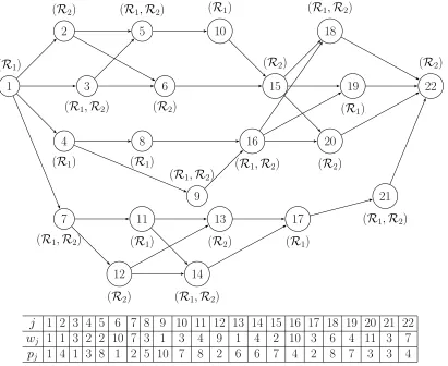
Figure 1.1 22-job network . . . 6

Figure 2.1 The system at stage _Ik . . . 19

Figure 2.2 At stage Ik with a decision to process job j[1] . . . 21

Figure 2.3 At stage _Ik with a decision to process job j[2] . . . 21

Figure 2.4 At stage Ik with a decision to process compatible jobs h j[2] j[1]i . . . 22

Figure 2.5 At stage _Ik with a decision to process job j[1,2] . . . 22

Figure 2.6 An example of initial set for 22-job network (Figure 1.1) . . . 24

Figure 2.7 An example of Re-sequencing procedure . . . 27

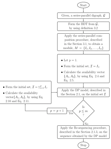
Figure 3.1 Series composition procedure flowchart . . . 40

Figure 3.2 Heuristic-DP (H-DP) algorithm flowchart . . . 42

Figure 3.3 Binary decomposition tree (BDT) of 22-job network (Figure 1.1) . 43 Figure 3.4 Final schedule of jobs on resources for 22-job network (Figure 1.1). 48 Figure 3.5 Jobs requiring resource R1 for 22-job network (Figure 1.1). . . 49

Figure 3.6 Jobs requiring resource R2 for 22-job network (Figure 1.1). . . 50

Figure 3.7 Jobs requiring resources (_R1, R2) for 22-job network (Figure 1.1). 51 Figure A.1 6-job network . . . 66

Figure A.2 9-job network . . . 67

(12)

Chapter 1 Introduction

1.1 Background

Scheduling problems are the class of optimization problems that deals with the allocation

of scarce resources (for example, processors or machines) to jobs, or tasks, over time.

These jobs may be related to each other by precedence relationships; that is, a job can

be processed only if all its predecessor jobs have completed their processing on their

respective resources, and the required resources are available for the current job.

Scheduling problems, especially those that require the simultaneous use of more than

one resource, arise in various areas such as manufacturing, production, service operations,

health care systems, and transportation, among others. Because of their importance,

scheduling problems have been extensively studied from the theoretical point of view

as well as their practical implementation. These problems are ubiquitous in the various

fields of engineering and management today, and indeed in everyday life experiences. For

example,

(13)

where a task needs to be processed by several processors simultaneously in order

to find a fault.

In the berth allocation problems at maritime ports, a large vessel (representing a task) may occupy several berths (representing a machine) for loading and/or

unloading.

In the planning of semiconductor circuit design workforce, a modular task is usually assigned to a team of people (representing aresources) to process the task (or jobs)

simultaneously.

In the car repair shops, a car has several broken parts that need to be repaired by one or more mechanics in the shop. These mechanics have to work on different

parts of the car in the order of their precedence; some parts need only one mechanic,

whereas others require more than one working simultaneously on the broken parts.

The car will leave the shop only when every broken part has been fixed.

A large number of practical problems similar to those mentioned above may be found

in different contexts; which existence motivated this research.

Similar to the other optimization problems, a scheduling problem also has two parts:

The first is theobjective function that one tries to optimize. In scheduling problems, typical objective functions are: minimize the weighted completion time of the jobs,

or the mean flow time, or the makespan (schedule length), or the total lateness of

the jobs (which presumes the existence of a due date for each job); and so forth.

The objective function is also called theperformance measure.

(14)

In the scheduling literature, the single resource scheduling problem is one of the most

extensively studied problems. There is a substantial body of work done on the scheduling

problem on a single resource, with or without precedence relations among the jobs, to

minimize the total weighted completion time ([4], [7], [14], [20], [21], [26]). However,

much less is known for more than one resource; only within the past two decades have

researchers addressed the multiple resource case. As expected, some of the work on the

single resource give valuable insights into the treatment of problems of more than one

resource.

Scheduling problems with precedence constraints are among the most difficult

prob-lems in the area of machine scheduling because of the impossibility of solving them

to optimality; either in polynomial time or with a known performance guarantee of an

approximate algorithm, which spills over to the difficulty in the design of good

approxi-mation algorithms. The understanding of the structure of these problems and the search

for their optimal or near-optimal solutions are continuing unabated in the operations

research field.

Historically, scheduling problems were the first problems to be analyzed for the study

of approximation algorithms. Garey et al [10] and later Johnson [16] formalized the

concept of an approximation algorithm. An approximation algorithm is evaluated by

its worst-case possible relative error over all possible instances of the problem, and is

necessarily executed in polynomial time. Formally an approximation algorithm for

min-imization, or maxmin-imization, of an objective function is defined as follows:

For minimization problems, an algorithmA is said to be a δ−approximation algo-rithm to problemP if for every instanceI ofP it delivers a solution that is at most

(15)

For maximization problems, a δ₋approximation algorithm delivers for every in-stance I of P a solution that is at least δ times the optimum. In this case δ < 1,

and the closer it is to 1, the better.

In the literature for the minimization problem,δis referred as theapproximation ratio,

orperformance guarantee, orworst case ratio, orworst case error bound, orapproximation

factor. Similarly, for the maximization problem 1/δ is referred to by any of these names.

The following points highlight the complexity of these problems and their solution

procedures.

The first approximation algorithm by Graham [12] for a single machine problem with precedence constraints to minimize the makespan (the completion time of the

last job), is still used for solving this problem.

The complexity of a problem of m (≥3) identical parallel machines with each job requiring a processing time of one time unit and the jobs are arranged by precedence

for the objective of minimizing the makespan is still an open problem as listed by

Garey et al [11].

For the problem of a single machine or m > 1 identical parallel machines with the objective of minimizing the weighted completion time, the constant-factor

ap-proximation algorithms were only developed over the last two decades ([18], [26]

etc.).

1.2 Statement of the Problem

(16)

switches over from one job to another and preemption is not allowed. A job j _{∈ N}, has one or more precedence relations; for example,j1, j2,andj3 are three jobs from the setN

such that j2 ≺ j1 and j2 ≺j3; where “≺” denotes precedence. The precedence relations

constitute a series-parallel (s/p) digraph (definition 2.2 or [30]). The processing time of

job j ∈ N, is a positive number pj > 0. Let Cj be the completion time of job j ∈ N. The objective is to find a feasible schedule that minimizes the total weighted completion

time, that is,

minX

j∈N

wjCj,

where wj ≥0 is the weight of job j ∈ N.

Figure 1.1 gives an illustrative example for a series-parallel digraph of 22 jobs with

resource requirement for each job shown next to each node, the weight and processing

time of each job are given in the table. Let j2 = 8, j1 = 16 and j3 = 9; then j2 ≺j1 and j3 ≺j1 shows an example of precedence relations for j1, j2,and j3 .

1.3 Problem Complexity

Hoogeveen et al [15] investigated the computational complexity of scheduling

multi-processor (or multi-resource) tasks (or jobs) with pre-specified multi-processor (or resource)

requirements. They investigated the complexity of a problem with the objective of

min-imizing the sum of the task (or job) completion times (i.e., wj = 1,∀j ∈ N in the objective function stated above), in the presence of precedence constraints. In their

pa-per the standard notation scheme of α _| β _| γ ([19]) was used to represent scheduling problem structure, where

(17)

1 (R1)

2 (_R2)

3 (R1,R2)

4 (R1)

5 (_R1,_R2)

6 (R2)

7 (R1,R2)

8 (R1)

9 (_R1,_R2)

10 (_R1)

11

(R1)

12

(_R2)

13

(R2)

14

(_R1,_R2)

15 (_R2)

16

(_R1,_R2)

17

(R1) 18 (_R1,_R2)

19

(R1)

20

(_R2)

21

(_R1,_R2) 22 (_R2)

j 1 2 3 4 5 6 7 8 9 10 11 12 13 14 15 16 17 18 19 20 21 22

wj 1 1 3 2 2 10 7 3 1 3 4 9 1 4 2 10 3 6 4 11 3 7

pj 1 4 1 3 8 1 2 5 10 7 8 2 6 6 7 4 2 8 7 3 3 4

Figure 1.1: 22-job network

number of resources (or processors). For example,α≡P3 refers to three processors (or resources).

β is the task (or job) characteristics. The notation β may denote either process-ing time of task (or job); or task (or job) requirements (that is, job j require

resource _R1 for processing, etc.); or the precedence relationship among jobs (that

is, series-parallel or no precedence, etc.); or any combination of processing time,

(18)

time unit.

γ represent the objective function; for example, γ _≡ PCj, where Cj is the com-pletion time of job j, is the total of completion time.

For instance, P m _|chain, f ixj, pj = 1| PwjCj refers to a scheduling problem with

m processors (or resources, denoted by P m) to minimize the total weighted completion

time (represented as PwjCj); where the processing time of job j is one time unit (that

is, pj = 1); the processor (or resource) allocated to job j is pre-specified (denoted by

f ixj; for example, job j require resource R1 for processing, etc.); and each job has at

most one predecessor and at most one successor (referred to as chain). They proposed a

total of 15 theorems; the two most important theorems, Theorem 3.3 and Theorem 3.6,

given below are closely related to this thesis.

Theorem 1.1(Theorem 3.3 from Hoogeveen et al [15]). TheP2|f ixj |PwjCj problem is N P−hard in the strong sense.

Theorem 1.2 (Theorem 3.6 from Hoogeveen et al [15]). The P2_| chain, f ixj, pj = 1 | P

Cj problem is N P−hard in the strong sense.

Both the Theorems 1.1 and 1.2 were proved based upon a reduction from 3₋partition. Combining both theorems, we get

Theorem 1.3. TheP2|chain, f ixj, pj = 1|PwjCj problem is N P−hard in the strong sense.

The problem of concern to us in this thesis,P2_|s/p, f ixj, pj |PwjCj,is a generaliza-tion of the problem considered in the Theorem 1.3; hence, the problemP2_|s/p, f ixj, pj | P

(19)

1.4 Literature Review

Since we focus on the objective of the total weighted completion time, we present here

what is known about this problem and what we consider to be the most relevant models.

For readers interested in scheduling theory in general, the book by Pinedo [22] is an

excellent recent text to consult. We have limited our studies to the objective of the total

weighted completion time because wj may represent either a holding cost per unit time

or the value already added to job j, both of which are of concern to management.

In deterministic scheduling theory, it has been typically assumed that each task is

processed by only one processor at a time. For the unconstrained single-machine problem

to minimize the sum of the weighted completion time, a simple interchange argument

proves that ordering the jobs according to non-decreasing pj/wj ratio is optimal; this

policy is known as Smith’s Rule as described in Smith’s paper [29]. When wj = 1,∀j; so that the objective is to minimize the sum of the (unweighted) completion times, Smith’s

rule says simply to process the jobs in the order of non-decreasing processing times (this

is the well-known SPT-rule).

The precedence constrained single-machine scheduling problem has attracted much

attention in the Operations Research community since Sidney’s [28] pioneering work in

1975. Sidney proposed a decomposition theorem (this is known asSidney’s decomposition

theorem) that partitions the set N of jobs into subsets or modules M1, M2, . . . , Mk (by using a generalization of Smith’s rule [29]); such that there exists an optimal schedule

where jobs from Mi were processed before jobs from Mi+1, for any i= 1, . . . , k−1.

Lawler [17] studied the problem of sequencing a set of n jobs on a single machine

subject to precedence constraints with the objective to minimize the total weighted

(20)

undirected graph _G = (_N,_A), the nodes of _G were assigned to integer points 1,2, . . . , n

on the real line to minimize the sum of arc lengths) into various versions of the sequencing

problems. He proved the _{N P−}completeness of the special cases of the problem under the arbitrary precedence: (i) when all job weights, wj = 1 and the processing time of

job j, pj ∈ {1,2,3}; and (ii) when the processing time of jobj, pj = 1 and the weight of job j, wj ∈ {k, k+ 1, k+ 2}, for any integer k.He also provided an elegant procedure of O(nlogn) for achieving the optimal sequence when the precedence relations result in a

series-parallel (s/p) graph.

It is very easy to find good feasible solutions; i.e., to obtain good upper bound on the

optimal value, to single machine scheduling problems, but it is very difficult to obtain

the tightest lower bound. The difficulty in finding optimal solutions, and the recent

advances in solving various combinatorial optimization problems via integer or mixed

integer programming (MIP), has encouraged many to study formulation of scheduling

problems as MIP modeling. Several MIP models and linear programming relaxations

have been proposed for this problem; which can be divided into three main groups based

on the decision variables used:

Dyer et al [8] exploit time-indexed variables, which are binary variables indicating when a job is completed. They derived various valid inequalities using time-indexed

variables in an MIP model to describe the convex hull of set of feasible solutions,

both in the absence of precedence constraints and in the presence of release dates

of jobs.

Balas [1] directly used the completion time variables in the presence of precedence constraints to obtain tight bounds for the Linear Programming (LP) relaxation.

(21)

indicate the order of job sequence, to obtain tight valid inequalities.

As mentioned above, LP relaxation in these three treatments has been applied to

ob-tain the constant-factor approximation algorithms. Hall et al [13] proposed time-indexed

LP relaxations that have (4 +)-worst case error bound approximation algorithms. A

weaker LP relaxations in completion time variables obtains 2-worst case error bound

approximation algorithm as shown by Schulz [27]. A LP relaxation in linear ordering

variables as suggested by Potts [23] can be used to obtain another 2-worst case error

bound approximation algorithm. Chudak et al [6] proposed a relaxation of Pott’s linear

program showing that the weaker linear program can be solved by one min-cut

compu-tation, which yields a combinatorial 2-worst case error bound approximation algorithms.

Chekuri et al [5] used Sidney’s decomposition theory to give an entire family of

combi-natorial 2-worst case error bound approximation algorithm.

Correa et al [7] discussed the problem of sequencing precedence-constrained jobs on

a single machine to minimize the total weighted completion time. They looked at the

problem from the polyhedral perspective, and presented a generalization of Sidney’s

results which leads to the conclusion that virtually all known 2-approximation algorithms

are consistent with Sidney’s decomposition theorem and belong to the class of algorithms

described by Chekuri et al [5]. They proved that the single-machine scheduling problem

with s/p precedence constraints is a special case of the vertex cover problem (given an

undirected graph G = (N,A), a subset C ⊆ N of nodes that minimizes the total weight

w(C) = P_j∈Cwj, for node weights wj ≥0,∀j ∈ N ).

In the last two decades, a great deal of work has been published in the scheduling

area that involves several resources working simultaneously to process jobs; and most

(22)

scheduling problem in which some jobs were processed by one machine while others were

processed by both machines simultaneously. They considered the objective of minimizing

the sum of the weighted completion times in the absence of precedence relationships.

The contribution of this paper are several. Regarding the complexity of the problem,

they use the 3-partition problem [11] (i.e., given a set S of 3n integers such that it can be partitioned into n disjoint subsets, each with 3 elements so that every subset has

exactly the same sum) to show that it is N P−complete in the strong sense. Optimality properties and a dynamic programming (DP) algorithm for the case of one two-processor

were presented. The DP algorithm finds the optimal solution in pseudo-polynomial time,

O(nT4_{) where}_T _{is the sum of all processing times and}_n_{is the number of jobs. They also}

claimed that the DP algorithm has a time complexity_O(nT3n2+1_{); where}_n

2(≥1) denotes

the number of jobs that require two-processors simultaneously. Heuristics methods that

can find approximate solutions efficiently were also proposed with 3₂-worst case error

bound.

Queyranne et al [26] considered the scheduling problem to minimize the sum of the

weighted completion times of n jobs on m identical parallel machines; where any job

j can be processed on any one of the machines, and a machine can process only one

job at-a-time. They considered both the precedence constraints and precedence delay

(i.e., if job i precede job j then job j can start after a delay, say dij time units, after

job j is finished) between jobs. They presented the best polynomial-time approximation

bounds for various scheduling problem; of which the most relevant to our problem are

wjCj; P m | prec., delay dij, pj = p | PwjCj; and 1 | prec., delay dij | PwjCj has worst case performance bounds of (4₋2/m), (3₋1/m), 4, 3 and 3; respectively.

(23)

related jobs on two resources to minimize the sum of the weighted completion times.

He used Elmaghraby’s procedure ([9]) to transform the non-s/p graph to a s/p graph.

The procedure introduce the artificial precedence relations (a.p.r.) into the precedence

graph to make it s/p graph and then reverse the relations to obtain the final sequence.

Since the reversal of the a.p.r.’s is of complexity 2m_, _where _m _{is the number of} _a.p.r.’s_;

which makes itN P−hard, a branch-and-bound approach was proposed to search in the solution space.

1.5 Organization and Outline

This thesis addresses the scheduling of precedence-constrained jobs on two resources (or

machines) in which a job may require either resource (or machine) or both, with the

objective of minimizing the total weighted completion time. In this chapter we have

presented a brief introduction to the scheduling problem of concern to us, the problem

description, the complexity of the problem and a concise review of the most relevant prior

contributions to our problem.

The remainder of the work presented in this thesis is organized as follows. In Chapter

2 we present the dynamic programming (DP) and the binary integer programming (BIP)

models while introducing the basic definitions and notation. We, first, develop and discuss

the DP model of the problem; then, formulate two BIP models of the problem, which

we label as the BIP and alternative-BIP (alt-BIP) formulations, and compare the time

taken by both the BIP and alt-BIP formulations to give an optimal solution. In Chapter

3, we present the Heuristic-DP (H-DP) algorithm that uses the DP model, discussed

in Chapter 2, to obtain feasible solutions, and illustrate H-DP algorithm with a 22-job

(24)

H-DP algorithm and use the BIP formulation to compare the results obtained. Chapter 4

summarizes the work presented in this thesis and presents the opportunities of future

(25)

Chapter 2 The Mathematical Models

In this chapter we present the two mathematical programming formulations that we

propose for the research problem of concern to us, namely,

1. the dynamic programming (DP) model, and

2. the binary integer programming (BIP) model.

We consider only the case of two resources (or machines), which are referred to as

R1 andR2; the three or more resources case may be approached in a similar fashion but

their practical solution is well beyond the capabilities of the models discussed here.

In discrete optimization problems oftentimes DP is used to obtain the solution. Since

DP is an enumerative algorithm, so in almost all cases the computational and data storage

requirements are overwhelming as the size of the problem increases, the size of the state

space becomes well beyond the capabilities of current computers (this is known as the

curse of dimensionality).

In general, the number of states in the DP approach grows exponentially in the

(26)

information. In truth, the curse of dimensionality in DP does not occur only due to the

state space; but also due to theoutput space and the action space; see the recent edition

of the book by Bellman [3] for further understanding the benefits and limitations of using

DP. Thus, generally speaking, direct application of DP is not a practical methodology

particularly for large-scale optimization problems. Hence, despite its mathematical

ele-gance and clarity, very few combinatorial optimization problems can be solved by the

direct application of the DP effectively.

We shall first present the DP formulation and then describe a method to reduce

the size of the state space. Many ingenious approaches such as Lagrange multipliers,

successive approximation, function approximation methods (e.g. neural networks, radial

basis representation, and polynomial representation) have been proposed to break the

curse of dimensionality, thus contributing diverse approximation DP methodologies to

the field of DP. Motivated by the need to address this curse of dimensionality several

researches have proposed approximations in DP. An excellent reference to learn more

about approximate dynamic programming (ADP) is the book by Powell [24].

Before presenting the DP formulation, we need to introduce some definitions and

notations, which we proceed to do.

We are given a directed acyclic digraph (dag), _G= (_N,_A); in which each nodej _{∈ N}

is identified as a job, and (i, j)_{∈ A} specifies the precedence relation between jobs i and

j; in particular, it implies that jobimust be completed before jobj can start, or in other

words, the directed path from job i to job j inG represents i≺j,∀i, j ∈ N, that is, job

i precedes job j.

Definition 2.1 (Transitive series-parallel;definition 1 in Valdes et al [30]):

(27)

The class of transitive series-parallel digraphs is defined recursively by a finite number

of applications of rules as follows:

1. A digraph _G consisting of a single node, for instance, _G = (_{i_}, φ) is transitive series-parallel.

2. If G1 and G2 are transitive series-parallel then G =G1× G2 is also transitive

series-parallel; whereN =N1∪N2, A=A1∪A2∪N1×N2.InG, i≺j, ∀i∈ N1, j ∈ N2;

that is, all nodes inG1 precedes every node ofG2; andN1×N2 refers to the directed

arcs joining the terminal nodes of _G1 with the start nodes of G2. G is said to be

formed by the series composition of _G1 and G2.

3. If _G1 and G2 are transitive series-parallel then G =G1∪ G2 is also transitive

series-parallel; where N =N1∪ N2, A =A1∪ A2.G is said to be formed by the parallel

composition ofG1 and G2. There is no precedence relationship between nodes ofG1

and G2 inG.

Definition 2.2 (Series-parallel (s/p) digraph; definition 2 in Valdes et al [30]):

A digraph _G is said to be series-parallel digraph, if and only if its transitive closure is transitive series-parallel (as described in definition 2.1).

So, the series-parallel precedence constraints are defined recursively with the base

elements as the individual jobs. Given series-parallel precedence relations by two digraphs

G1 = (N1,A1) and G2 = (N2,A2) such that N1 ∩ N2 = φ. The parallel composition of

G1 and G2 results in a partial order on N1∪ N2 that maintainsA1 and A2,but does not

introduce any additional precedence relationships. The series composition of _G1 and G2

(28)

Definition 2.3 (Initial set):

The set of initial jobs, that is, those jobs with no predecessors, is called an initial set;

denoted by _{I ⊆ N}.

Definition 2.4 (Eligible set):

The subset of jobs in initial set_I available to be processed immediately on their required resources is called the eligible set; denoted by_{E ⊆ I ⊆ N}.

For example, let I ={1,2}and 1≺2; the only job that is available for processing is job number 2, so _E =_{2_}.

Definition 2.5 (Marginal cost):

The marginal cost of a set I, denoted byρ(I), is defined as

ρ(I) = P

j∈Iwj P

j∈Ipj

(2.1)

where wj ≥0 is theweight, or value and pj >0 is the processing time of job j,∀j.

Clearly, ρ(I) is well-defined becausepj >0,∀j.

Definition 2.6 (Compatible job pairs):

Two jobs are said to be acompatible job pairs if each of them requires a different resource

and can be processed concurrently (they have no precedence relationship).

The jobs in a compatible job pair may be processed in parallel (because they have no

precedence relationship) and can be considered as one job that requires more than one

resource at the same time. In particular, if jobsj[1] and j[2] require resources R1 and R2

respectively, then the compatible job pair, denoted by h_j [2] j[1]i

(29)

given by

ρh_j

[2] j[1]i

= wj[1]+wj[2] max_{pj[1], pj[2]}

(2.2)

This approach of forming a compatible job pair is found useful, as is explained in

chapter 3, since it helps in reducing the state space of the DP.

Definition 2.7 (Compatible set):

The set of job pairs formed from the eligible set E, by pairing all possible compatible jobs (obtained by following definition 2.6) is called the compatible set; denoted by _C.

For example, suppose that the eligible set is E ={j[1], j[2], k[2]},where jobj[1] requires

resource R1; job j[2] and job k[2] require resource R2 each. Then, the compatible set

is C = nh_jj_[2][1]i,h_k

[2] j[1]io

; where the marginal cost of each compatible job pair can be

calculated by Eq. 2.2.

Definition 2.8 (Composite job):

Two or more jobs may be grouped together to constitute a composite job if they are

precedence related consecutively in series and they share at least one resource among

them. Their marginal cost is evaluated following Eq. 2.2.

For example, suppose that we have two jobs: j(1) _and _j(2)_{, where job} _j(1) _requires

resource R1, written as j_[1](1) and job j(2) requires both resources R1 and R2, written as j_[1(2)_,_2]; then the composite job, denoted by k , j_[1](1), j_[1(2)_,_2], will have a marginal cost

(using definition 2.5) given by,

ρ(k) =

w_j(1) [1]

+w_j(2) [1,2]

p_j(1) [1]

+p_j(2) [1,2]

(30)

Definition 2.9 (Directed cut, definition from Provan et al [25]):

A directed cut in a directed network; _G = (_N,_A) with a source node s _{∈ N} and sink note t _{∈ N}, is a set of arcs of the form (_N1,N2) ={(n1, n2) : n1 ∈ N1, n2 ∈ N2}; where s_{∈ N}1 and t∈ N2 =N − N1.

Definition 2.10 (Uniformly directed cut (udc), definition from Provan et al [25]):

A uniformly directed cut is a directed cut (_N1,N2) for which (N2,N1) is empty.

In words, auniformly directed cutset is a set of arcs such that each path in the network

contains exactly one arc in it.

0 A1

R1 j[1,2] j[1]

R2 j[1,2] j[2]

0 A₂

Figure 2.1: The system at stage _Ik

2.1 A Dynamic Programming (DP) Formulation

2.1.1 The elements of Dynamic Programming

Stage: The stage of the system is the initial set _Ik (definition 2.3), in which the subscript k identifies the stage number. For example, Figure 2.1 exhibits one such

stageIk of the system; wherej[1], j[2] and j[1,2] are the jobs that needs resource R1,

resourceR2,and both resources (R1,R2), respectively.

State: At stage _Ik, let s(Ik) = (A1, A2) denote the state of the system. In

(31)

and A2 represents the total time taken by all the jobs in the initial set Ik to be processed on resources _R1 and R2, respectively. We need to enumerate both A1

and A2 over all possible values of their availabilities. They are bounded by alower

bound (l.b.) and anupper bound (u.b.) as follows:

X

j[1]∈Ik

pj[1] ≤A1 ≤ X

j[.]∈Ik

pj[.] (2.4)

X

j[2]∈Ik

pj[2] ≤A2 ≤ X

j[.]∈Ik

pj[.] (2.5)

where j[.] denotes those jobs that need either resource R1, or resource R2, or both

resources_R1andR2;j[1]andj[2]are jobs that need resourceR1andR2 respectively.

Decision: From the eligible set _Ek (which is a subset of the initial set Ik), there may be four different possibilities of jobs immediately available to process; they

are,

1. jobs, j[1],that require only resource R1,

2. jobs, j[2],that require only resource R2,

3. compatible jobs h_j [2] j[1]i

that require resources _R1 and R2,

4. jobs, j[1,2], that require both resources R1 and R2.

The decision at the stage_Ikis generically designated by dk,which implies to sched-ule the job(s) specified by dk.

Extremal Equations:Letf_{Ik,(A1, A2)}denote the minimal cost when in stage

Ik (the initial set Ik) is scheduled to terminate at (A1, A2).

(32)

1. If the decision is to process job j[1] ∈ Ek ⊆ Ik on resource R1 that would

terminate (that is, finish) at timeA1,as shown in Figure 2.2, giving the stage

reward of wj[1]A1 for stage Ik; then the cost in stage Ik is

f{Ik,(A1, A2)}= min

j[1]∈Ek⊆Ik{

wj[1]A1 +f{Ik\{j[1]},(A 0

1, A2)}};

whereA0

1 =A1−pj[1].

0 A0₁ A₁

R1 j[1]

R2

0 A₂

Figure 2.2: At stage Ik with a decision to process job j[1]

0 A₁

R1

R2 j[2]

0 A0₂ A₂

Figure 2.3: At stage _Ik with a decision to process job j[2]

2. If the decision is to process job j[2] ∈ Ek ⊆ Ik on resource R2 that would

terminate (that is, finish) at timeA2,as shown in Figure 2.3, giving the stage

reward of wj[2]A2 for stage Ik; then the cost in stage Ik is

f{Ik,(A1, A2)}= min

j[2]∈Ek⊆Ik{

wj[2]A2 +f{Ik\{j[2]},(A1, A 0

(33)

whereA0

2 =A2−pj[2].

3. If the decision is to process compatible jobs h_jj_[2][1]i on resources R1 and R2

that would terminate (that is, finish) job j[1] and job j[2] at time A1 and A2

respectively, as shown in the Figure 2.4, giving the stage reward of wj[1]A1+

wj[2]A2 for stageIk; then the cost in stageIk is

f{Ik,(A1, A2)}= _"min

j[2] j[1]#

∈Ck

{wj[1]A1+wj[2]A2+f{Ik\{j[1], j[2]},(A 0

1, A

0

2)}};

whereA0

1 =A1−pj[1] and A

0

2 =A2−pj[2].

0 A0₁ A₁

R1 j[1]

R2 j[2]

0 A0₂ A₂

Figure 2.4: At stage Ik with a decision to process compatible jobs h

j[2] j[1]i

0 A₁ A0₁ Amax

R1 j[1,2]

R2 j[1,2]

0 A0₂ A₂

Figure 2.5: At stage _Ik with a decision to process job j[1,2]

4. If the decision is to process job j[1,2] ∈ Ek ⊆ Ik on both resources R1 and R2

that would terminate (that is, finish) at time Amax= max{A1, A2}, as shown

(34)

cost in stage_Ik is

f_{Ik,(A1, A2)}= min

j[1,2]∈Ek⊆Ik{

wj[1,2]Amax+f{Ik\{j[1,2]},(A 0

max, A

0

max)}};

whereAmax = max{A1, A2} and A0max=Amax−pj[1,2].

Hence, the minimal cost, f{Ik,(A1, A2)}, in stage Ik scheduled to terminate at (A1, A2) is given by the extremal equations given below:

f{Ik,(A1, A2)}= min

                

wj[1]A1+f{Ik\{j[1]},(A 0

1, A2)}, (2.6)

wj[2]A2+f{Ik\{j[2]},(A1, A 0

2)}, (2.7)

wj[1]A1+wj[2]A2+f{Ik\{j[1], j[2]},(A 0

1, A

0

2)}, (2.8) wj[1,2]Amax+f{Ik\{j[1,2]},(A

0

max, A

0

max)} (2.9)

with f_{φ,(A1, A2)}= 0

whereA0

1 =A1−pj[1], A

0

2 =A2−pj[2], Amax= max{A1, A2},andA 0

max =Amax−pj[1,2].

Given a digraph _G= (_N,_A), it is easy to find the initial set, _Ik ⊆ Nk, by generating all possible uniformly directed cuts (udc‘s). Once an _Ik is identified, the availability vector (A1, A2) can be calculated using Eq. 2.4 and Eq. 2.5. The computational challenge

encountered here is the problem of dimensionality of the state variable,s(Ik) = (A1, A2),

since we need to enumerate all feasible values of the vector (A1, A2) of each initial setIk. For the 22-job network given in Figure 1.1, we exhibit one such initial set with 13

jobs to get the initial setI ={1,2,3,4,5,6,8,9,10,15,16,18,19},as shown in Figure 2.6. Using Eq. 2.4 and Eq. 2.5 to calculate the l.b. and u.b., as shown in the Figure 2.6, it is

(35)

enumerated for this stage of the DP procedure. Evaluating all possible values of

availabil-ity vector (A1, A2) becomes computationally burdensome to the point of intractability; so

we need to explore a systematic procedure to reduce (or better bounding) the availability

vector (A1, A2).

1 (R1)

2 (_R2)

3

(_R1,R2)

4

(_R1)

5 (_R1,R2)

6

(_R2)

8

(_R1)

9

(R1,R2) 10 (_R1)

16

(_R1,R2) 15 (_R2)

18 (_R1,R2)

19

(R1)

Lower Bound,l.b.(Ai) Upper Bound,u.b.(Ai) Cardinality ofAi,|Ai|=u.b.(Ai)−l.b.(Ai) + 1

A1 54 66 13

A2 43 66 24

13_×24 = 312 different vectors of (A1, A2).

(36)

2.2 New lower and upper bounds on resource

avail-ability

Let the availability of resources R1 and R2 obtained by solving the DP for Ik−1 be

denoted byA(₁k−1) and A₂(k−1) respectively. Then the new lower bound (nlb) and thenew upper bound (nub) of Ai’s required to solve the DP from initial set Ik are given by:

nlb(Ai) = A(k

−1)

i +

X

j[i]∈Ik\Ik−1

pj[i],∀i (2.10)

nub(Ai) = A(k

−1)

i +

X

j[.]∈Ik\Ik−1

pj[.],∀i (2.11)

where, j[i] is the job that requires resource Ri, i = 1,2; and j[.] is the job that require

one or both resources taking precedence and compatible jobs into account. Clearly, this

should reduce the vector space of resource availability (A1, A2) by a significant amount

as we are using availability information from a previously solved DP stage.

2.3 The Re-sequencing Procedure

The objective of this procedure is to correct the case in which the DP results in the

scheduling of a compatible jobs that violates some precedence relation.

Suppose that at stage _Ik, the availability of resourcesR1 and R2 are A1 and A2,

re-spectively. Suppose, further, that the only decision is to process the compatible jobsh_j [2] j[1]i

from the eligible set _Ek (definition 2.4). Then, in the next stage k+ 1; the availabilities are A0

j[1] =A1−pj[1] andA 0

(37)

k[2] k[1]

from the eligible set Ek+1(⊆ Ik+1); the application of the DP procedure will result

in the sequence shown in the Figure 2.7(b). Clearly, this is not a feasible solution because

job k[1] precedes job j[2]; so j[2] cannot be processed on resource R2 before job k[1] has

finished processing on resource _R1. It is at this point that the re-sequencing procedure

(38)

0 A

0j_[1]

A

j_[1]

R

1

j

[1]

R

2

j

[2]

0 A

0j_[2]

A

j_[2]

(a) The compatible job pairs

  _j

[2] j_[1]





are allocated.

0 A

0k_[1]

A

0j_[1]

A

j_[1]

R

1

k

[1]

j

[1]

R

2

k

[2]

j

[2]

0 A

0k_[2]

A

0j_[2]

A

j_[2]

(b) The compatible job pairs

  _k

[2] k_[1]





are allocated; but

k

_[1]

≺

j

_[2]

0 A

0k_[1]

A

0j_[1]

A

j_[1]

R

1

k

[1]

j

[1]

R

2

k

[2]

j

[2]

0 A

0k_[2]

A

k_[2]

A

0j_[2]

A

j_[2]

(c) Applying re-sequencing procedure on the sequence in (b).

(39)

Let the final sequence of jobs generated after the completion of the DP procedure be

denoted by Υ, which is used as an input to the re-sequencing procedure to get a feasible

and better solution.

1. Initialize a sequence, denoted by Ω,with no jobs; that is, Ω ={φ}.The correspond-ing availability vector on resourcesR1 and R2 is (A1, A2) = (0,0).

2. Allocate one-by-one jobs (this include jobs that require only one resource _Ri, i= 1,2 or both resources (_R1,R2)) or compatible jobs as sequenced in Υ to resources

R1 and R2 by considering precedence relationship, and append those job(s) to

the sequence Ω accordingly. At each step, calculate the availability vector (A1, A2)

based on the precedence relationship.

3. Use the availability vector (A1, A2) to calculate the completion time of each job j,

denoted by Cj; which is the sum of starting time and processing time of job. The

completion time, Cj,is used to obtain the total weighted completion time.

For example, suppose the final sequence (Υ) of jobs generated after the completion

of the DP procedure is shown in Figure 2.7 (b). By applying there-sequencing procedure

to Figure 2.7 (b), in the final feasible sequence (Ω), job j[2] starts on resource R2 only

after job k[1] has finished processing on R1, as shown in Figure 2.7 (c).

2.4 A Binary Integer Programming (BIP)

Formula-tion

LetA={< j, j0 _>_|_{j, j}0 _{∈ N }}_{be the set of pairs of jobs related by immediate}

(40)

N, _N[2] ⊆ N and N[1,2] ⊆ N respectively.

Also, let the upper bound ofcompletion time of the last job beTmax,which is the sum

of processing time of all jobs, that is,Tmax=P_j∈N pj. The minimum processing time of

all jobs in _N is denoted bypmin = minj∈N{pj}.

Let xjt be a binary variables, for j ∈ N and t ∈[0, Tmax−pmin], such that

xjt =       

1 if job j starts at time t,

0 otherwise.

(2.12)

Also, let Cj be the completion time of job j,∀j ∈ N.

The binary integer programming (BIP) formulation for the problem is as follows:

z = minX

j∈N

wjCj (2.13)

subject to

1. a job j _{∈ N} must start at some time t_∈[0, Tmax−pmin]:

TmaxX−pmin t=0

xjt = 1 (2.14)

2. the completion time of job j is the sum of its start time at t and the processing

time pj:

Cj =

TmaxX−pmin t=0

(t+pj)·xjt (2.15)

(41)

only after job j1 is finished:

Cj1 ≤Cj2 −pj2 (2.16)

4. for all pairs, < j1, j2 > /∈ A and < j2, j1 > /∈ A,∀j1 ∈ N[1,2] and j2 ∈ N(j1 6=j2) :

Either, a job j1 requiring both resources (R1,R2) must be finished before job j2

can be processed:

Cj1 ≤Cj2 −pj2 (2.17)

Or, a job j2 must be finished before job j1 that require both resources (R1,R2)

can be processed:

Cj2 ≤Cj1 −pj1 (2.18)

5. for all pairs, < j1, j2 > /∈ A and < j2, j1 > /∈ A,∀j1, j2 ∈ N[i](j1 6=j2) :

Either, a job j1 requiring resource Ri must be finished before any job j2 can be

processed on the same resource _Ri :

Cj1 ≤Cj2 −pj2 (2.19)

Or, a job j2 must be finished before jobj1 requiring resourceRi can be processed:

Cj2 ≤Cj1 −pj1 (2.20)

6. binary variable conditions:

xjt ∈ {0,1} (2.21)

Note. CPLEX gives the functionality to model Either-Or constraints; for example,

(42)

described above, without having to reformulate BIP into standard MIP (Mixed Integer

Programming) formulation.

In the standard MIP formulation for BIP model described above, we rewrite Equations

(2.17); (2.18); (2.19); and (2.20) as follows.

Letyj1j2 be an indicator variable such that

yj1j2 =       

1 if Eq. 2.17 is constraining and Eq. 2.18 is always satisfied,

0 otherwise, i.e., Eq. 2.18 is constraining and Eq. 2.17 is always satisfied. (2.22)

Cj1 ≤Cj2 −pj2 +M ·(1−yj1j2) (2.23)

Cj2 ≤Cj1 −pj1 +M ·yj1j2 (2.24)

where, M =Tmax.

Similarly, letyj1j2 be an indicator variable such that

yj1j2 =       

(43)

Cj2 ≤Cj1 −pj1 +M ·yj1j2 (2.27)

where, M =Tmax.

Note. The total number of binary decision variable,xjt,of this BIP model forn jobs will be [n(Tmax−pmin) +n]; which depends on the processing time of jobs. If the processing

time of every jobsj is multiplied with a factor of 10; the total number of binary decision

variable will increase by [9n(Tmax−pmin)].

The BIP formulation described above is one way of formulating the problem. We will,

also, introduce an alternative BIP (alt-BIP) formulation and compare the time taken to

obtain the optimal solutions by the BIP and the alt-BIP formulations in the Table 2.1.

The objective function (minPwjCj), the decision variables (xjt) and some of the

constraints (Eq. 2.14, Eq. 2.15, Eq. 2.16, and Eq. 2.21) of the BIP formulation will also

be the objective function, the decision variables and constraints of the alt-BIP

formula-tion. Hence, to avoid the repetition we will only present the constraints of the alt-BIP

formulation that differs from the BIP formulation; that is, only those constraints that

corresponds to the item numbers 4 and 5 of the BIP formulation (the constraints - either

Eq. 2.17 or Eq. 2.18, and either Eq. 2.19 or Eq. 2.20):

4. for all pairs, < j1, j2 > /∈ A and < j2, j1 > /∈ A,∀j1 ∈ N[1,2] and j2 ∈ N(j1 6=j2) :

Either, a job j1 requiring both resources (R1,R2) must be finished before job j2

can be processed:

t1xj1t1 +pj1 ≤t2xj2t2 +Tmax(1−xj2t2),∀t1, t2 (2.28)

(44)

can be processed:

5. for all pairs, < j1, j2 > /∈ A and < j2, j1 > /∈ A,∀j1, j2 ∈ N[i](j1 6=j2) :

Either, a job j1 requiring resource Ri must be finished before any job j2 can be

processed on the same resource _Ri :

Or, a job j2 must be finished before jobj1 requiring resourceRi can be processed:

Similar to the BIP formulation, the constraints either (2.28) or (2.29); and either

(2.30) or (2.31) of the alt-BIP formulation can be rewritten as follows:

Letyj1j2 be an indicator variable such that

yj1j2 =       

(45)

t2xj2t2+pj2 ≤t1xj1t1 +Tmax(1−xj1t1) +Tmaxyj1j2,∀t1, t2 (2.34)

Similarly,

yj1j2 =       

t1xj1t1 +pj1 ≤t2xj2t2 +Tmax(1−xj2t2) +Tmax(1−yj1j2),∀t1, t2 (2.36)

t2xj2t2+pj2 ≤t1xj1t1 +Tmax(1−xj1t1) +Tmaxyj1j2,∀t1, t2 (2.37)

We solved the five instances of 6-job network (Figure A.1 (i)) with the BIP and

alt-BIP formulations to see the time it takes to give an optimal solution; Table 2.1 shows

the time performance comparison between them. The alt-BIP formulation takes more

time to obtain an optimal solution compared to the BIP formulation. Since, the alt-BIP

has large number of constraints (corresponding to the item numbers 4 and 5, that is,

constraints either Eq. 2.33 or Eq. 2.34; and either Eq. 2.36 or Eq. 2.37 ) compared to the

BIP formulation; which leads to sparse matrix.

Table 2.1 shows that CPLEX takes much longer amounts of computational time for

the alt-BIP formulations due to the sparsity of matrix. It is possible to resolve the issue of

sparse matrix by applying theDelayed Column generation or the Dantzig Wolfe

decom-position, or theBender’s Decomposition technique; however, in this research work we are

(46)

Table 2.1: Comparison between the BIP and alt-BIP formulations

Network Objective function value Time (in seconds)

Instance BIP alt-BIP BIP alt-BIP

I.6.1 654 654 0.23 3.95

I.6.2 489 489 0.23 0.59

I.6.3 567 567 0.23 5.36

I.6.4 303 303 0.27 1.17

I.6.5 925 925 0.29 14.73

Since, we observe that the computation time is less for the BIP formulation compared

to the alt-BIP formulation; so we use the BIP formulation to compare the results achieved

(47)

Chapter 3 The Heuristic-DP Algorithm

In this chapter we will first define the relevant terms such as thejob module and thebinary

decomposition tree; then, present theSeries-parallel Composition procedure which is used

to generate the initial setsIk(definition 2.3). We will, then, summarize the steps involved in obtaining the solution to the problem by the DP model into one algorithm, which we

call it as theHeuristic-DP (H-DP) algorithm. We briefly show, with an example of 22-job

network, the steps involved in the H-DP algorithm to obtain the solution. Finally, we will

perform experiments by taking various instances of different problem sizes and discuss

the results in Section 3.5.

Definition 3.1 (Module; definition 1 in Lawler [17]):

Let M be a subset of _N. A nonempty subset M is a (job) module if, for each job

j _{∈ N −}M, exactly one of the following three conditions holds:

1. j _≺k, _∀k_∈M, that is,j must precede every job inM;

2. j k, _∀k_∈M, that is,j must follow every job inM;

(48)

Definition 3.2 (Binary decomposition tree (BDT)):

Given a series-parallel digraph _G, a binary decomposition tree (BDT) of _G, is a rooted binary tree obtained by repeatedly applying rules of transitive closure on_G,as described in the definition 2.2, to decomposing _G into series-parallel components. Each internal node of the BDT has at most two descendants (hence the binary in the name).

Each leaf of the BDT is identified with a node of _G.Each internal node is marked ‘S’ indicating the series composition of the subgraphs identified with its two descendants,

with the convention that the left descendant precedes the right one. Each internal node

marked ‘P’ indicates the parallel composition of the subgraphs identified with its two

descendants. The subscripting in ‘S0_{s’ and ‘}_P0_{s’ are to facilitate reference for creating}

modules as detailed later.

In the paper by Valdes et al [30], a procedure is described to determined if a digraph

G is series-parallel and, if it is, the procedure to obtain its BDT. This task can be accomplished on _O(m +n) running time, where m is the number of arcs and n the number of nodes of _G. Hence, we shall always have a BDT for a given series-parallel precedence constraints.

3.1 The Procedure Based on the BDT

The series composition procedure described here emulates the algorithm described in

Lawler’s paper [17] for finding an optimal sequence for a moduleM by series composition

from previously determined optimal sequences for its descendants,M1 andM2. But in the

parallel composition procedure, a slight modification is considered to form a compatible

job (as defined in definition 2.6) whenever feasible.

(49)

each module M from the previously determined sequences of its descendants, M1 and

M2. At the end of the procedure, the module M is arranged in non-increasing order of

ratios ρ (definition 2.5).

3.1.1 Series Composition

Step 0: Assume thatM1 contains a dummy element,d1; with marginal cost,ρ(d1) = +∞;

and that M2 contains a dummy element, d2; with marginal cost, ρ(d2) = −∞. The

assumption of dummy elements is required to avoid the test for emptiness in the steps

that follow.

Step 1: Take the minimal element i∗ _from _M

1 (which must be the last element, by

construction) and the maximal element j∗ _from_M

2 (which must be the first element, by

construction).

Step 1.1: If ρ(i∗₎_{> ρ}₍_j∗₎_, _{then form}_M ₌_M

1∪M2 such thati≺j, ∀i∈M1 ⊆M

and _∀j _∈M2 ⊆M; that is, the moduleM1 precedes the module M2 in the module

M. Stop the algorithm and exit.

Step 1.2: Else (i.e., ρ(i∗₎_≤_ρ₍_j∗_{)) remove} _i∗ _from _M

1; i.e., M1 ←M1\{i∗}, and j∗

from M2; i.e., M2 ←M2\{j∗}, to form the composite job pair k ←(i∗, j∗). Go to

Step 2.

Step 2: Take the minimal element i∗ _from_M

1, which is the last element, by

construc-tion.

Step 2.1: If ρ(i∗₎ _{> ρ}₍_k₎_, _{in which job} _k _{is the one formed in Step 1, then go to}

(50)

Step 2.2: Else (i.e.,ρ(i∗₎

≤ρ(k)) removei∗ _from_M

1; i.e.,M1 ←M1\{i∗},and form

the composite job pair k_←(i∗_{, k}_{); then go to Step 2.}

Step 3: Take the maximal element j∗ _from _M

2, which is the first element, by

con-struction.

Step 3.1: If ρ(k) > ρ(j∗₎_, _{in which job} _k _{is the one formed in Step 2, then form}

M =M1∪ {k} ∪M2 such that i≺k ≺ j, ∀i∈M1 ⊆M and ∀j ∈M2 ⊆M; that

is, the module M1 precedes the job k which then precedes the module M2 in the

module M. Stop the algorithm and exit.

Step 3.2: Else (i.e., ρ(k) _≤ ρ(j∗_{)) remove} _j∗ _from _M

2; i.e., M2 ← M2\{j∗}, and

form the composite job pair k _←(k, j∗_{); then go to Step 2.}

At the end of series composition procedure the module M is a sequence obtained by

listing the jobs, arranged by non-increasing order of ratios,ρ(definition 2.5). The dummy

elements d1 and d2 are removed from the final module M.

Figure 3.1 show the series composition procedure described above in a flowchart

rep-resentation

Note. Eitheri∗_, _or_j∗_, _{or both may, by themselves, be composite jobs; so the composite}

job, k, represents a sequence formed by joining together the two sequences represented

byi∗ _and _j∗_.

3.1.2 Parallel Composition

For parallel composition of job modulesM1 andM2, arrange the elements of M1 and M2

(51)

Start

Let d1 ∈ M1 andd2 ∈ M2; whereρ(d1) = +∞and ρ(d2) =−∞

(Step 0)

Leti∗ _{= arg min}

i∈M1ρ(i)

andj∗ _{= arg max}

j∈M2ρ(j).

(Step 1)

Is ρ(i∗₎_{> ρ(j}∗₎

?

(Step 1.1)

M1 ← M1\{i∗}andM2 ← M2\{j∗}

Form the composite pair,k ←(i∗, j∗) (Step 1.2)

i∗ _{= arg min}

i∈M1ρ(i)

(Step 2)

M1 ← M1\{i∗} Form the composite

pair,k ← (i∗, k)

(Step 2.2)

Is ρ(i∗₎ _{> ρ(k)}

?

(Step 2.1)

j∗ _{= arg max}

j∈M2ρ(j)

(Step 3)

Is ρ(k)> ρ(j∗)

?

(Step 3.1)

M = M1∪M2

(Step 1.1)

M =M1∪ {k} ∪M2

(Step 3.1)

M2 ← M2\{j∗} Form the composite

pair,k ← (k, j∗)

(Step 3.2) Stop No Yes No Yes No Yes

(52)

assuming that feasibility is true for M1 and M2 individually. For the job pair j[1] and j[2]

form a compatible job,h_j [2] j[1]i

, if it is feasible.

Later in this chapter the need to form compatible jobs will make more sense;

essen-tially, this operation helps in reducing the state space of the DP model.

3.2 The Heuristic-DP (H-DP) Algorithm

Given an acyclic series-parallel (s/p) digraph _G,

Step 1: Form the BDT for G using the definition 3.2.

Step 2: Apply the Series-parallel Composition Procedure, described in the Section 3.1, to the BDT to obtained amodule arranged in non-increasingρ (definition 2.5).

Step 3: Use the DP model explained in section 2.1 to secure the preliminary se-quence of the jobs in_G.

Step 4: Apply the Re-sequencing procedure, describe in the Section 2.3, to obtain the availability vector (A1, A2) and the total weighted completion time.

Figure 3.2 shows the H-DP algorithm described above in flowchart representation.

3.3 An Example of the H-DP Algorithm

(53)

Start

Given, a series-parallel digraph,

_G

Form the BDT from

_G

,

by using definition 3.2

Apply the series-parallel

com-position procedure, described

in the Section 3.1, to obtain a

module,

M

=

_{

I

1

, I

2

, . . . , I

m

}

• Let p = 1.

• Form the initial set,

_I

=

I

1

.

• Calculate the availability vector

{

A

1

, A

2

}

, by using Eq. 2.4 and

Eq. 2.5.

Apply the DP model, described in

the Section 2.1, on the initial set

_I

• Form the initial set,

_I

=

Ppi=1

I

i

.

• Calculate the availability

vector

_{

A

1

, A

2

}

,

by using Eq.

2.10 and Eq. 2.11.

Is

p

_≤

m

?

p

=

p

+ 1

Apply the Re-sequencing procedure,

described in the Section 2.1.3, on the

sequence obtained by the DP model

Stop

Yes

No

(54)

S21

1 S20

P19

S12

P9

S3

S2

4 P1

8 9

16

S8

P4

2 3

S7

P6

S5

5 10 6

15

P11

P10

18 19

20

S18

S16

7 S15

P13

11 12

P14

13 14

S17

17 21

22

(55)

Applying the Series-parallel Combination procedure, described in the section 3.1, we

finally get a module M21 = {I1, I2, I3, I4}, (see the steps to obtain M21 in Appendix C)

where

I1 = (1,7,3), I2 = (2,6), I3 =

h

12

11i

,

I4 =

4,8,9,16,5,10,15,h₂₀19i,18,14,13,17,21,22

with ratios ρ(I1) = 2.75, ρ(I2) = 2.2, ρ(I3) = 1.625, ρ(I4) = 0.775.

Now, the module M21 is partitioned into subsets Sk = ∪ki=1Ii, ∀k; which is used as the initial set to start the DP procedure (described in the section 2.1).

1. The initial set isI1 =I1 ={1,7,3}with the final availability vector (A1, A2) having

nlb(A1) = 1 + 2 + 1 = 4,nub(A1) = 1 + 2 + 1 = 4

nlb(A2) = 0 + 2 + 1 = 3,nub(A2) = 1 + 2 + 1 = 4

The extremal equation of the DP is

f1 =f{I1,(A1, A2)}= min

d {wdAd+f{I1\{d},(A

0

1, A

0

2)}}

Solving the extremal equation and applying the re-sequencing procedure results

in the sequence of processing jobs, _{1,7,3_}, as shown in Figure 3.4(a) and its availability vectorA∗

1 = 4 andA∗2 = 4 with the objective function value f1 = 34.

2. The initial set is I2 = I1 ∪ I2 = {1,7,3,2,6} with the final availability vector

(A1, A2) having

nlb(A1) = A∗1+ 0 = 4,nub(A1) =A∗1+ 4 + 1 = 4 + 5 = 9

(56)

f2 =f{I2,(A1, A2)}= min

d {wdCd+f{I2\{d},(A

0

1, A

0

2)}}

Solving the extremal equation and applying the re-sequencing procedure, one can

obtain the sequence of processing jobs,_{1,7,3,2,6_},as shown in Figure 3.4(b) and its availability vectorA∗

1 = 4 andA∗2 = 9 with the objective function valuef2 = 132.

3. The initial set is I3 = I1∪I2∪I3 = {1,7,3,2,6,11,12} and the final availability

vector (A1, A2) having

nlb(A1) = A∗1+ 8 = 4 + 8 = 12, nub(A1) = A∗1+ 8 = 4 + 8 = 12

nlb(A2) = A∗2+ 2 = 9 + 2 = 11, nub(A2) = A∗2+ 8 = 9 + 8 = 17,

because compatible job pair,h₁₂11ischeduled at the same time sopj = max{p11, p12}=

8.

f3 =f{I3,(A1, A2)}= min

d {wdCd+f{I3\{d},(A

0

1, A

0

2)}}

Solving the extremal equation and applying the re-sequencing procedure, one can

obtain the sequence of processing jobs, n

1,7,3,12,2,h11₆ io, as shown in Figure 3.4(c) and its availabilities A∗

1 = 12 and A∗

2 = 11 with the objective function value f3 = 256.

Scheduling Precedence-Constrained Jobs On Two Resources To Minimize The Total Weighted Completion Time.

ABSTRACT

DEDICATION

BIOGRAPHY

ACKNOWLEDGEMENTS

TABLE OF CONTENTS

LIST OF TABLES

LIST OF FIGURES

Chapter 1

Introduction

1.1

Background

1.2

Statement of the Problem

1.3

Problem Complexity

1.4

Literature Review

1.5

Organization and Outline

Chapter 2

The Mathematical Models

2.1

A Dynamic Programming (DP) Formulation

2.1.1

The elements of Dynamic Programming

2.2

New lower and upper bounds on resource

avail-ability

2.3

The Re-sequencing Procedure

0

A

A

R

j

R

j

0

A

A

(a) The compatible job pairs

are allocated.

0

A

A

A

R

k

j

R

k

j

0

A

A

A

(b) The compatible job pairs

are allocated; but

k

≺

j

0

A

A

A

R

k

j

R

k

j

0

A

A

A

A

(c) Applying re-sequencing procedure on the sequence in (b).

2.4

A Binary Integer Programming (BIP)

_G

_G

_{

_I

_I

_I

_{

_≤