Methodology and accuracy of estimation of quantitative trait loci parameters in a half-sib design using maximum likelihood.

Copyright 0 1995 by the Genetics Society of America

Methodology and Accuracy of Estimation of Quantitative Trait Loci Parameters

in a

Half-sib

Design

Using

Maximum Likelihood

M. J. Mackinnon"

and

J. I. Welled

*Institute of Cell, Animal and Population Biology, University of Edinburgh, Edinburgh EH9 3p, United Kingdom and +Institute of Animal Sciences, Agricultural Research Organization, The Volcani Centre, 50250, Israel

Manuscript received February 15, 1995

Accepted for publication June 27, 1995

ABSTRACT

Maximum likelihood methods were developed for estimation of the six parameters relating to a marker-linked quantitative trait locus (QTL) segregating in a half-sib design, namely the QTL additive effect, the QTL dominance effect, the population mean, recombination between the marker and the QTL, the population frequency of the QTL alleles, and the within-family residual variance. The method

was tested on simulated stochastic data with various family structures under two genetic models. A

method for predicting the expected value of the likelihood was also derived and used to predict the lower bound sampling errors of the parameter estimates and the correlations between them. It was

found that standard errors and confidence intervals were smallest for the population mean and variance,

intermediate for QTL effects and allele frequency, and highest for recombination rate. Correlations among standard errors of the parameter estimates were generally low except for a strong negative

correlation ( r = -0.9) between the QTL's dominance effect and the population mean, and medium

positive and negative correlations between the QTL's additive effect and, respectively, recombination

rate ( r = 0.5) and residual variance ( r = -0.6). The implications for experimental design and method

of analysis on power and accuracy of marker-QTL linkage experiments were discussed.

D

ETECTION of major genes influencing quantita-

tive traits is now feasible with the explosion of

genetic marker technology in recent years. DNA-level

markers can be used to establish genetic maps and sys-

tematically screen genomes for quantitative trait loci

(QTL) in many agriculturally important species (ED-

WARDS et al. 1987; PATERSON et al. 1988; FRIES et al.

1989; HALEY et al. 1990; KEIM et al. 1990; SOLLER 1990; GEORGES et al. 1995). Detection of QTL can be achieved

by finding a difference in quantitative trait value of two

groups of offspring inheriting alternative marker alleles

from a common heterozygous parent. This procedure

can be used for both inbred species (e.g., experimental

species such as Drosophila and mice) using crosses be-

tween inbred lines (SAX 1923; SOLLER et al. 1976) and

for outbred species (e.g., farm animals and fruit trees)

where the analysis is carried out within large family

groups ( GELDERMANN 1975; NEIMANN-SBRENSEN a n d

ROBERTSON 1961; SOLLER a n d GENIZI 1978).

Having detected a QTL, it is of interest to find its

location in the genome by estimating its recombina-

tion distance from the marker and to determine the

effects of the QTL in the population by estimating the

magnitude of its effect, the degree of dominance, and

its frequency in the population. All of these parame-

ters are important for both assessing the potential use-

Corresponding author: Margaret Mackinnon, Institute of Cell, Animal

and Population Biology, University of Edinburgh, West Mains Rd., Edinburgh, EH9 3JT, UK. E-mail: eangZO@festival,ed.ac.uk

(knrtics 141: 755-770 (October, 1995)

fulness of the QTL in genetic improvement programs

and the way in which it will be used. Estimation of

these parameters can be carried out using maximum likelihood methods. While the power to detect QTL has been described well for both inbred line cross de-

signs (SOLLER et al. 1976; WELLER 1986, 1987; JENSEN

1989; LANDER a n d BOTSTEIN 1989; LUO and KEARSEY 1989; SIMPSON 1989; KNOTT a n d HALEY 1992a; DARVASI

et al. 1993) a n d within-family designs (SOLLER and

GENIZI 1978; WELLER et al. 1990; KNOTT a n d HALEY 199%; BOVENHUIS and WELLER 1994), only a few stud-

ies have explored the accuracy of the estimates (KNOTT

a n d HALEY 1992a,b; VAN OOIJEN 1992; DARVASI et al.

1993). All of the latter have relied on replicated sto- chastic simulations to measure accuracy empirically.

As this can be tedious, it would be useful to be able

to predict the accuracy of QTL parameters using theo-

retical methods, although the complex nature of the

likelihood models has so far prevented this being

done. In this study, a quasitheoretical numerical

method is used to predict both power and accuracy of QTL parameters from the shape of the multidimen-

sional expected likelihood surface. It is applied to the

half-sib design in which six parameters are estimated

simultaneously and is used to explore the effects of

data structure, statistical model and inaccurate marker

allele frequencies o n power, accuracy and sampling

correlations between parameter estimates. The proce-

dure described here can be used to determine the

to extract the best information marker-QTL linkage data.

THEORY

Experimental design: There

about the QTL from

are s sires each of

which produce Nprogeny when mated to an outbred population of dams. The phenotype for a quantitative trait is determined by many genes of small effect and

by random environmental factors, which together

cause the trait to be normally distributed with a mean

of p and variance of 0’. The trait is also affected by

a relatively major QTL with two alleles, Q and q, at

population frequencies of

p

and 1 -

p,

respectively.

Additive and dominance effects at the QTL are de-

noted a and d, respectively. Thus there are three possi-

ble genotypes, QQ

Qq

and

qq,

which have quantitative

trait values of pQQ = p

+

a, pQ(! = p

+

d and pUeu = p

- a. A marker locus is situated adjacent to the QTL

at a recombination distance of r. Only sires heterozy-

gous for the genetic marker are included in the analy- sis. The notation will assume only two alleles at the

genetic marker, M and m, although a situation of mul-

tiple marker alleles can be handled with only minor modifications. Thus sires have one of four possible

marker-QTL genotypes, viz: M W m Q M U mq, Mq/ mQ

or Mq/mq. Dams have one of 10 possible genotypes corresponding to all possible combinations of gametes

M Q Mq, mQ and mq. The frequency of allele M in the

dam population is denoted t and is assumed to be

known or estimated with a high degree of accuracy. The population is assumed to be at Hardy-Weinberg equilibrium with respect to the QTL and marker locus.

Progeny with records are assumed to be a random

sample of the sire’s progeny with respect to their value for the quantitative trait and marker loci.

Likelihood of the model: The likelihood for the half-

sib design, first given by WELLER (1990) and extended

here to account for dominance, QTL allele frequency and marker allele frequency, is

3 x , 3

L =

fi

[ d

n

n

c

C i l f ( X k - pl)

b i = l k = l I

6 nz_J 3

+

p(1

-

p )

n n

C , j f ( X k - pj) i=4 k = l 1

9 s

+

p(1

-

p )

n n

c i f f ( x k - pj) 1=7 k = l 1

+

(1 -

n n

c t f f ( x k - pj) ( l )

I2 n1-9 3

z = I O k = l j

1

where b = 1 to s and denotes the family number, i =

1-12 for progeny marker genotypes of M M , M m and

mm nested within sire marker-QTL genotypes M W m Q

M W m q , Mq/mQand Mq/rnq, respectively; nt = the num- ber of progeny in the ith marker genotypic group and

ni = nz+3;

j

= 1 , 2 and 3 for progeny QTL genotypes

QQ

Qq

and qq, respectively; cq = the element in row i

and column

j

from the matrix, C (Table 1) , of progeny

QTL genotype probabilities conditional on sire QTL

genotype and progeny marker genotype; and f( xk - pJ

= the normal density function for the kth observation, xk, ( k = 1,

. . .

, n,) of the bth sire of the ith marker genotype group, conditional on the jth QTL genotype,

and is abbreviated by and calculated as:

e-l/2cx,-y/oP

&0

.

A

= f ( x k - p,) =

The four terms that are summed in the likelihood

equation for each sire represent the four possible

QTL genotypes of the sire, denoted h. That is, for

each possible genotype of the sire, the statistical den- sity of the sire’s progeny’s genotypes, conditional on

this sire’s genotype, is computed over all the observed

data. These terms, called sublikelihoods from here on, are multiplied by the probabilities of the sire’s

genotype Ph

[p2

for h = 1,

p (

1 -

p )

for h = 2 or 3 and

(1 -

p)*

for h = 41 and summed to obtain the overall

likelihood.

C, the matrix of progeny QTL genotype probabilities,

conditional on sire QTL genotype and progeny marker genotypes and assuming linkage equilibrium is com-

puted as shown in Table 1. The rows of C represent the

progeny marker genotypes, MM, Mm, and mm, nested

within sire marker-QTL genotype, as shown to the right

of the matrix. The columns of C represent the progeny

QTL genotypes

QQ

Qq, and

qq.

Thus the probabilities

for each row sum to unity.

Each sire passes on average half of his breeding value

for the quantitative trait to his progeny. Equation 1

does not account for variance among sires due to genes

other than the QTL. The likelihood was therefore mod-

ified by subtracting half the sire’s polygenic breeding

value, g b , from each observation. Estimates of the sire’s

breeding value from genetic evaluations based on infor- mation from ancestors and descendants will include the

sire’s QTL genotype effect and are therefore biased

estimates of gb. Thus an alternative estimate of g b is

required. For the situation here, where each sire has

many offspring, an appropriate estimate is g b = x b - Gh

where

x,,

is the observed mean of the sire’s progeny

and Gh is the expected QTL genotype mean of the sire’s

progeny, which is a function of a, d and

p

(BOICHARD

et al. 1990). This is likely to be an effective way of parti-

tioning out the effects of polygenes from the QTL effect

in the sires because it uses two pieces of good and

almost independent information, namely the sire

mean, which estimates the total genetic effect, and the between-marker contrast within this sire mean, which

estimates the QTL effect. Because gb is conditional on

the sire’s QTL genotype, it is different for each of the

four summed terms of (1). The likelihood accounting

Estimation of QTL Parameters 757

TABLE 1

Progeny QTL genotype probabilities conditional on sire marker-QTL genotype and own marker genotype

C =

-

Progeny QTL genotype

Progeny marker Sire

Q4 44 genotype genotype

MM

M m M W m 4

MM mm

P

p

+

r - 2pr l - p - r + P mm

P

p

+

r - 2pr l - p - r + p r M M

[ t P ( l - [ t ( l -

p

- r

+

2pr) [ t ( l - p ) r

+ ( I - t , p l + ( 1 - t ) ( p

+

r - 2pr)l + ( I - t ) ( 1 -

p

- r

+

r p ) ] Mm M d m Q

P ( 1 -

4

l - p - r + 2 f w (1 - p ) r mm

0

P

1 - P MM

0

P

1 - P M d m 4 M m

0

P

1 - P

_-

mm

i=10 k = l f

The properties of this likelihood were explored both

by computation of its expectation as a function of pa-

rameter estimates (deterministic simulations) and by stochastic simulations. The situations for which simula-

tions were performed are summarized in Table 2 and

described in more detail below.

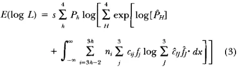
Deterministic simulations: Expectation of the log likeli-

hood: A close approximation of the expected value of

the natural log likelihood, E(1og L ) , for a given set of

parameter estimates is obtained by modifymg (1) to

give the following equation:

4

h

The derivation of this equation and the degree of approx-

imation is explained in the APPENDIX. Note that now the

lowercase subscripts h, iandjindicate that the parameters

are the true values and the uppercase superscripts and the indicate that these parameters are estimates or func- tions of estimates on which the value of the likelihood is

conditional. Thus the symbols in (3) take on the follow-

ing meanings: h denotes the sire's true QTL genotype,

and H the sire's hypothesized QTL genotype; Ph denotes

the expected frequency of sires with genotype h in the

data (depending on the real value of

p,

as described

above), and P H denotes the probability that the sire has

genotype H, which is a function of the current estimate

of

p ,

denoted

p?

ttris the conditional probability of falling into the@ QTL class and the fth marker-sire class given

the current estimates of the parameters

p

and r, denoted

p

and and the hypothesized sire genotype, H, where

Z

= i - 3 h

+

3H;J is an abbreviation of the density function

defined previously used in (1) and (2) depending on

whether the model takes account of polygenic effects

(see below) and

f j

is the function

fi

given the estimates

of their component parameters e.g, t43 = (1 -

fl

and n,

is the expected number of observations in the ith marker

genotypic group and is equal to '/?Nt, for i = 1, 4,

7,

and

10; '/&for i = 2, 5, 8, and 11; and '/2N(l - t ) for i =

3, 6, 9, and 12, respectively. Without polygenic effects

(Equation

I),

=

A x k

- p j ) and J?i = f ( x k - j l j ) . With

polygenic effects (Equation

21,

J = f ( x k pl - &) and

f j

= f i x k - j l J - g b ) where gb = gb - -

G.

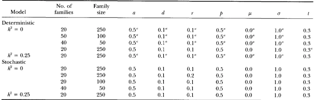
TABLE 2

Models, family structures and parameter values used for simulations

No. of Family

Model families size a d r

_P

_P

U t

Deterministic

h2 = 0 20 250 0.5'' 0.1" _{0.1" 0.5" 0.0" 1 .Of'}

50 100 0.5" 0.1" 0.1" 0.5" 0.0" 1 .Of'

0.3

40

0.3 50 0.5" 0.1" 0.1" 0.5" 0.0" 1 .0"

20 250 0.5 0.1 0.1 0.5 0.0 1 .0 0.3"

0.3

h' = 0.25 20 250 0.5" 0.1" 0.1" 0.5" 0.0" 1 .Of' 0.3

h2 = 0 20 250 0.5 0.1 0.1 0.5 0.0 1 .0 0.3

20 250 0.5 0.1 0.2 0.5 0.0 1.0 0.3

20 100 0.5 0.1 0.1 0.5 0.0 1.0 0.3

40 50 0.5 0.1 0.1 0.5 0.0 1.0 0.3

h' = 0.25 20 250 0.5 0.1 0.1 0.5 0.0 1 .0 0.3

h' = 0 indicates that the data were simulated without polygenes; hz = 0.25 indicates that the data were simulated with polygenes,

Stochastic

which accounted for 20% of the residual variation.

The likelihood was evaluated for a range of parameter estimates around these true values.

because it is based on infinite sample size theory, is

equivalent to the average of the log L evaluated in an

infinite number of replicates of stochastic data. It is

therefore useful for examining the shape of the log L

surface in infinite samples. Because it is the shape of

the surface around the maximum which determines the

accuracy of the parameter estimates, this method is thus a useful tool for exploring the properties of the likeli- hood surface without having to resort to many time- consuming replicates using stochastic data. The popula-

tions used in this study are large but not infinite, in

which case the expected log L is an approximation to

the true average likelihood. In the size of data sets used in this study, this approximation appears to be close enough to have no appreciable influence on the power

and accuracy (see APPENDIX).

Shape of the likelihood surface: Equation 3 was evaluated

for values of estimates f i , 6,

d,

?,

j ,

and 8 , which ranged

from +0.25 of the true values p = 0, a = 0.5, d = 0.1,

r = 0.1,

p

= 0.5 and n = 1 in increments of 0.025 for

three family structures ( N = 250, s = 20; N = 50, s =

100; N = 40, s = 50) without a polygenic effect in the

model and one structure ( N = 250, s = 20) with a

polygenic effect in the model (Table

2).

These data

structures and parameter values are considered to be typical of large-scale studies likely to be used for map- ping QTL in forest trees or animals. The marker allele

frequency, t, was 0.3 in all cases. For each parameter

varied, all other parameters were held at their true val-

ues. In these simulations gb was set to 0 because for

deterministic evaluations, this parameter is, in effect,

known. log L was then plotted against each parameter

to give "uniparameter profile likelihoods" assuming all other parameters are known. Three-dimensional plots

of log L as a function of two parameters were also pro-

duced for a few pairs of parameters ( 6 and

d,

d

and ?,

fi

and

d)

to examine the shape of the likelihood surface

with respect to these parameters for the presence of

ridges or local maxima.

Accuracy of the estimates: From the uniparameter pro-

file likelihoods, the 95% confidence intervals were cal-

culated as the parameter value at which the log I,

equalled the maximum log L (log &) plus half the 95%

chi-squared value

(x2)

on one degree of freedom ( i . ~ . ,

log I,,,, = log

4,

+

1.92). This test statistic is based on the fact that for large samples, the difference between

log L maximized for all but one parameter (log L , ) ,

and log L maximized for all parameters (log &,) is as-

ymptotically distributed as

-'/&

with one degree of

freedom (WILE 1938). Assuming normality of the esti-

mate's sampling distribution, the standard error of the

estimate is expected to be half the 95% confidence

interval (KENDALL and STUART 1973). Approximate

standard errors and the correlations between them

were also calculated from the approximate variance-

covariance matrix of the estimates, which is obtained from the inverse of the matrix of all the second partial

derivatives of the log likelihood function ( i . e . , the ob-

served information matrix) (KENDALL. and STLJART

1973). These are lower bound standard errors ac-

cording to the Cramer-Rao inequality. For the simula- tion conditions used above, these second derivatives

were obtained by evaluating (3) at points on the surface

at small distances (?0.005) away from the true values

for all possible pairwise combinations of the parame- ters. This matrix was then inverted to give the approxi- mate variances and covariances of the parameter esti- mates and from these the standard errors of the

estimates and correlations between them were calcu- lated. When the matrix of numerically derived second

derivatives was not positive definite, the interval at

Estimation of QTL Parameters 759

in cases where the matrix was positive definite for both intervals, indicating that the choice of interval size did not have detectable effects on the results. The estimates of standard errors derived from the information matrix differ from those calculated from the confidence inter- vals by the fact that they are not based on the assump- tion that all other parameters are known. To test the effect on the accuracy of a single parameter of fixing

all other parameters us. simultaneously estimating all

parameters, standard errors were calculated from the reciprocal of only the diagonals of the information ma- trix instead of the inverse of the whole matrix. This effectively ignores any covariances between parameters. Standard errors derived in this way and those derived from the confidence intervals are called “uniparameter

standard errors” from here on, and those derived from

the full information matrix are called “multiparameter standard errors”.

Effect of marker allele frequency: The effect of using

wrong values of the marker allele frequency, t, was inves-

tigated by replacing t with

i

ranging from 0 to 1 in

intervals of 0.1 in ( 3 ) . Maximum likelihood estimates

of each of the parameters were found while holding all other parameters constant. The bias in each parameter over the range of iwas calculated.

Stochastic simulations: Stochastic simulations were performed to illustrate that estimates of all parameters could be obtained by numerical maximization in sto- chastic data. Also the results from stochastic simulations were used to compare with those from the deterministic simulations. Data on progeny from multiple half-sib families of equal size were generated by first randomly assigning QTL genotypes to sires according to probabil-

ities

p’, p(

1 -

p ) ,

p(l

-

p )

and (1 -

p)2,

and then

generating progeny from each sire by random sampling from independent normal distributions with means of pj ( j = 1, 2 or 3 for QTL genotypes QQ

Qq

or

qq)

and

variance u2 in the expected proportions given the sire’s

genotype and frequency of the QTL alleles in the dam population. Marker genotypes were then assigned at

random according to expected frequencies given the

progeny’s QTL genotype. Three different family sizes

( N = 50, 100, and 250), two numbers of families (s =

20 and

40)

and two recombination rates ( r = 0.1 and

0.2) were simulated (Table

2).

The other parameters

were set at p = 0, a = 0.5, d = 0.1,

p

= 0.5, u = 1 and

t = 0.3. The above simulations assumed that, except for

the linked QTL, sires all had equal breeding values. A

further simulation with N = 250, s = 20, r = 0.1, p =

O , a = 0 . 5 , d = 0 . 1 , p = 0 . 5 , ~ = 1 a n d t = 0 . 3 , w a s performed accounting for polygenes by adding a half of a sire value randomly sampled from a normal distri-

bution with mean of 0 and variance 1/4uz = 0.0625 ( i e . ,

h2 = 0.25). Because random mating between sires and

dams was assumed, it was not necessary to account for genetic variation among dams for polygenes.

Fifteen replicate populations were generated for each

combination of values. For each replicate, maximum

likelihood estimates of ( p a ) , ( p

i-

d), ( p A a ) , f,

j

and 6 were obtained by numerically maximizing the

logarithm of the likelihood described in (11, [or

(2)

for the simulations with a polygenic effect] using the iterative numerical maximization subroutine GEMINI

(LALOUEL 1979). This routine guarantees to find the global maximum and extensive testing using different starting values on same sets of data indicated that s t o p ping at local maxima was extremely unlikely. Thus for the replicates reported here, prior values were chosen at random from a range spanning the possible parame- ter space given the limits imposed by the overall mean and variance of the observed data. Convergence was considered to be reached when the normalized gradi-

ent of the likelihood was

<lop5.

Parameters were con-

strained to wide boundaries, and in the case of r and

p,

were allowed to go out of the theoretical parameter

space during iterations to facilitate convergence. If con- vergence was reached at values outside the parameter space, iteration was restarted with a different set of pri- ors. Standard errors were estimated from the inverted matrix of the numerically derived second derivatives of

the function close to the maximum (LALOUEL 1979).

Predicted standard errors of combined parameters

were calculated from the predicted variances and co- variances of individual parameters. For example, the

standard error of ( p

I

a) was calculated as the square

root of the sums of the squared standard errors of ci

and

b

plus twice the covariance between them.

For all replicates the likelihood was also maximized

with rfixed at r = 0.5 to obtain a

x:

statistic with which

to test the null hypothesis of no linkage between the

marker and the QTL. As stated above, the four terms

which are summed in the likelihood equations (1) and

(2) represent the four possible QTL genotypes for each

sire. The most likely QTL sire genotype was designated as that corresponding to the maximum of the four sub- likelihoods.

RESULTS

Deterministic simulations: All of the deterministic

simulations performed in this study took <5 min to

run on a personal computer with a 80486 processor.

Thus the method was very rapid and not limited by

computer requirements.

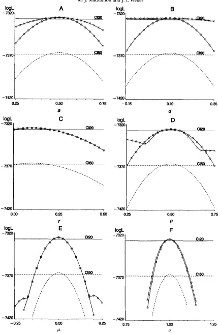
Standard errors from conJidence intervals: Figure 1 shows

the log L profiles as functions of each of the six parame-

ters

b,

ci,

2,

f,

fi

and 6 for two family structures (20 X

250 and 50 X 100) with and without a polygenic effect.

The likelihood always maximized at the true value of the parameters indicating that the expected value of

the log likelihood as given in (3) calculated using deter-

ministic simulation yielded unbiased maximum likeli-

hood estimates, despite it being an approximation. Also

shown in Figure 1 are the confidence intervals ( a 2 0

M. J. Mackinnon and J. I. Weller

A

logL

B

0.25 0.50 0.75 -0.15 0.10 0.35

a d

0.00 0.25 0.50

r

0.25 0.50 0.75

P

I /

-

V[''

''\\\\\,\,\\L

-

/!

.

7370 """""- """"-~"")c""""- "" """""

7370 """""""

""","'.""

"

I \

-

7420 '\ J:

_-

₇₄₂₀

-0.25 0.00 0.25 0.75 1.00 1.25

P u

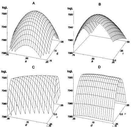
FIGURE 1.-Uniparameter profiles of the expected log likelihood (log L ) with respect to parameter estimates assuming all other parameters known for data sets with 5000 records divided into either 20 families without (0-0) and with (X-X) a polygenic effect fitted in the model o r 50 families (-

-

- -) without a polygenic effect. True values of parameters were a = 0.5, d = 0.1, r = 0.1,

p

= 0.5, t = 0.3, p = 0 and g = 1. Confidence intervals for estimates from data with 20 families (CI20) and

Estimation of QTL Parameters 761

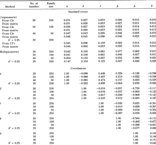
TABLE 3

Standard errors and correlations from deterministic simulations No. of Family

Method families size ci

2

i?

P

P

B

Uniparameter

From CIS

From matrix

From CIS

From matrix

From CIS

From matrix

From CI's From matrix

Multiparameter

h2 = 0.25

h2 = 0.25

h' = 0.25

h2 = 0.25

h2 = 0.25

h2 = 0.25

h2 = 0.25

20 50 40 20 20 50 40 20 20 50 40 20 20 50 40 20 20 50 40 20 20 50 40 20 20 50 40 20 250 100 50 250 250 100 50 250 250 100 50 250 250 100 50 250 250 100 50 250 250 100 50 250 250 100 50 250

Standard errors

0.031 0.027

0.031 0.028

0.030 0.027

0.031 0.028

0.047 0.043

0.048 0.045

0.045 0.098

0.046 0.098

0.042 0.100

0.041 0.100

0.064 0.159

0.147 0.104

Correlations

1

.oo

-0.096 1

.oo

-0.088 1

.oo

-0.085 1

.oo

-0.282 1

.oo

1

.oo

1

.oo

1

.oo

0.053 0.053 0.053 0.053 0.085 0.086 0.103 0.053 0.061 0.061 0.097 0.122 0.448 0.467 0.474 0.898 -0.016 -0.016 0.017 -0.243

1

.oo

1

.oo

1

.oo

1

.oo

0.026 0.027 0.024 0.025 0.046 0.046 0.022 0.020 0.077 0.049 0.056 0.027 0.329 0.218 0.157 -0.064 -0.057 -0.037 -0.026 0.012 -0.020 -0.013 -0.009 -0.087

1

.oo

1

.oo

1

.oo

1

.oo

0.015 0.015 0.014 0.015 0.023 0.023 0.014 0.015 0.063 0.057 0.086 0.020 -0.128 -0.022 0.023 0.039 -0.759 -0.863 -0.908 -0.005 0.025 0.020 0.018 0.058 -0.564 -0.402 -0.298 -0.677

1

.oo

1

.oo

1

.oo

1

.oo

0.010 0.01 1 0.011 0.011 0.019 0.019 0.012 0.01 1 0.013 0.013 0.021 0.029 -0.538 -0.536 -0.535 -0.920 -0.117 -0.122 -0.123 0.187 -0.354 -0.357 -0.358 -0.850 -0.112 -0.072 -0.051 0.069 0.163 0.140 0.131 -0.043

Uniparameter and multiparameter lower bound standard errors of parameter estimates, and correlations between them,

derived from deterministic simulations for various models and family structures. True parameter values were p = 0.0, a = 0.5,

d = 0.1, r = 0.1,

p

= 0.5, o = 1 and h' = 0, unless otherwise indicated. around the maximum likelihood estimates. The stan-

dard errors derived from these confidence intervals

(uniparameter standard errors), and those for the 40

sires X 50 progeny structure (not shown in Figure 1)

are given in Table 3. Clearly, r is the most difficult

parameter to estimate accurately because of the flatness of the likelihood surface across the range of values (Fig-

ure 1C) and largest standard error. The profile likeli-

hoods for 2,

d

and

fi

were all similar in curvature (Figure

1, A, B and D) and had similar confidence intervals, indicating that these parameters are estimated to ap- proximately the same degree of accuracy. The profiles

for /i and b were steepest reflecting the greater informa-

tion contributing to these parameters (Figure l , E and

F). The effect of decreasing total experimental size

from 5000 to 2000 was to increase the standard errors

by -50% for all parameters except forb. The effect of increasing the number of families on accuracy of all parameters was negligible. Allowing for a polygenic ef- fect in the model seemed to decrease the accuracy of

2 and

d,

increase the accuracy of

p

and do nothing to

the accuracy of ?, jl, and 8, although these effects could

not be tested for statistical significance. The reduction

M. J. J. I.

35

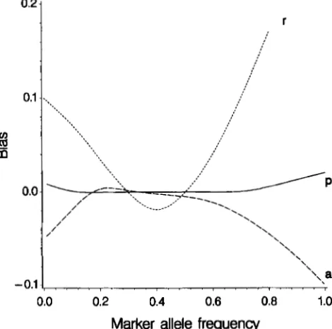
FIGURE 2.-Expected log likelihood surface with respect to estimates of two parameters at a time. (A-C): No polygenic effect was fitted whereas in D it was. Data sets comprised 5000 records divided into 20 families with true parameter values of a = 0.5,

d = 0 . 1 , r = 0 . 1 , p = O . 5 , t = 0 . 3 , p = O a n d a = l .

by estimating the polygenic effect, g b , as a function of

the sire’s major genotype mean, G b , this conditions out

some of the information on the component parameters

of this mean,

ci,

d,

and

$.

While this explains the de-

crease in accuracy of ci and

8,

it is not clear why the

accuracy of

$

increases when this polygenic effect is

included. Accuracies of ?, ji, and 6 are not affected by

the incorporation of a polygenic effect because these

parameters are not components of the adjustment

term, g b .

Standard errors and correlations from the information ma-

trix: Approximate standard errors of the estimates un-

der the four sets of deterministically simulated condi-

tions (Table

2)

and the matrix of correlations between

them are given in Table 3. Uniparameter standard er-

rors derived from the diagonals of the information ma- trix were similar to those derived from the confidence intervals from the profile likelihoods. The multiparame- ter standard errors were considerably higher than the

uniparameter standard errors, indicating that confi-

dence intervals derived from profile likelihoods gener- ated by assuming all other parameters are known will

overestimate the accuracy of the estimates from a mul-

tiparameter model when the parameter estimates are

not independent, i.e., correlated. While in general

there were low correlations between parameter esti- mates across the range of conditions tested, there were some notable exceptions: a high correlation (-0.9) be-

tween jl and

d,

and medium correlations (50.4 to 0.6)

between 6, ?and 6. This first correlation is presumably

because when

p

= 0.5, none of the between-marker

contrasts are influenced by d so that the information

on d relies on the mean of the M m group of progeny

from heterozygous sires. This mean has an expectation of ( p

i

’/&)

so that

d

and jl are confounded. This

correlation is expected to be lower when

p

is not equal

to 0.5 because the between-marker contrasts then be-

Estimation of QTL Parameters 763

this correlation is reduced to -0 because the expecta-

tion of the mean becomes jl

+

1/2d

+

- ‘ / 2 d = jl

+

&.

Thus

d

and

fi

are no longer confounded. The

correlations between 6, Pand 6 arise from the fact that

the contrast yielding most information on these param-

eters is MM vs. mm, which has an expected value of (1

- 2 r ) a / o . Thus high values of ci are consistent with

high values of P and low values of 6. These correlations

become higher ( a 20.9) when much of the informa-

tion on ci is conditioned out by accounting for the poly-

genic effect. Even though these correlations exist and influence the accuracy of the estimates, the fact that they are not perfect indicates that there is some inde-

pendent information contributing to each parameter

and thus each of the parameters is, in theory, estimable. These results show that the accuracy of individual pa-

rameter estimates is partly dependent on the data struc-

ture and partly on the statistical model fitted to the data.

Figure

2

shows three-dimensional representations of

the likelihood surface with respect to two parameters

at a time (ci and

d,

ci and P, jl and

4.

The figures

illustrate that the surface is relatively uniform in curva- ture and has a single global maximum. This indicates that, in theory at least, the approach to the maximum during the estimation procedure should be relatively

unimpeded. Figure 2, C and D, shows the relationship

between

0

and

2

with and without a polygenic effect

fitted, respectively. It can be seen that while there is a

ridge along the axis of

d

in both figures, that the orien-

tation of the ridge when the polygenic effect is not

fitted (Figure 1C) is on the diagonal of jl and dwhereas

it is almost parallel with

d

when a polygenic effect is

fitted (Figure 1D). This reflects the dependence be-

tween jl and

d

in the first case and their independence

in the second case. Similarly, the orientation of the

profiles for ci and

2

in the same plane as their corre-

sponding axes in Figure lA, and the slightly diagonal

orientation of the profiles for P in Figure l B , respec-

tively, reflect the independence and moderate depen- dence between these pairs of parameters. Thus these three-dimensional figures are useful to illustrate the behavior of maximum likelihood estimators in multipa- rameter models.

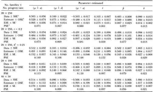
Effect of wrong marker allele frequency: Figure 3

shows the bias in estimates of ci, ? and

j

as functions

of assumed marker allele frequency,

f,

when the true

frequency was t = 0.3. It was found that P was very

sensitive to f, always being inflated by wrong allele fre-

quencies, 6 was moderately sensitive, and always de-

flated, and

fi

was relatively unaffected. There were no

effects on d,

0

and 6. Thus inaccuracies in estimated

marker allele frequencies will cause the QTL to appear smaller and less tightly linked than it really is. The mag- nitude of the bias in recombination fraction was of the

order of one standard error in the case presented here.

Stochastic simulations: Stochastic simulations were

performed on a Sun SparcStation 2 computer. On this

O.*l r

,

-0.1 , , , , , , , , , , , , , , , , , , , , , , , , ,

‘\,a

0.0 0.2 0.4 0.6 0.8 1

.o

Marker allele frequency

FIGURE 3.-Bias in estimates of 2, i and as functions of

assumed marker allele frequency,

6

for data sets of 5000 rec-

ords divided into 20 families and true parameter values of a = 0 . 5 , d = 0 . 1 , r = 0 . 1 , p = 0 . 5 , t = 0 . 3 , p = 0 0 n d u = l .

machine, which processes at 2.4 X

lo6

floating point

operations per second, a typical run time per replicate

for 30 iterations or -350 evaluations of the likelihood

on 5000 records was -6 min of CPU. Generally only

one run was required for a replicate to reach conver-

gence, although -10% of runs had to be restarted with

different starting values because of parameters esti-

mates exiting the parameter space.

Estimates and standard mors: The estimates from the simulations, averaged over replicates, are given in Table 4. The success in obtaining estimates similar to simu- lated values shows that the half-sib likelihood model

presented in (1) and (2) can separate the effects of the

individual parameters and that estimation by numerical maximization is computationally feasible. Close agree- ment between the means over replicates of simulated and estimated parameter values indicates that the esti-

mates were unbiased or at least that any bias was negligi-

ble (Table 4). This applied equally in models with and without the polygenic effect, indicating that the method of approximating and adjusting for the polygenic ef- fects was successful in separating the major (QTL) ge- notype effect from polygenic effects.

Standard errors of the estimates are also given in

Table 4. These standard errors are derived from various

sources. The standard error on the simulated data repli-

cate mean (SSE) simply reflects the variation between

replicates in the true parameters due to sampling in

the simulated data and is based on only 15 observations.

The standard error on the estimated parameter (OSE)

is also based on 15 observations and is the observed

between-replicate variation in estimates of the parame-

J. Mackinnon and J. Weller

TABLE 4

Parameter estimates and standard errors from stochastic simulations

No. families X Parameter estimated

No. progeny/sire ( P

4

( P

4

( P

4

5

P

B

20 X 250 Data ? SSE"

Estimate t OSEh

ESE ? SE'

PSE"

20 X 250, r = 0.2 Data ? SSE

Estimate ? OSE

ESE ? SE

PSE

20 X 250, hz = 0.25 Data +- SSE

Estimate ? OSE

ESE ? SE

PSE 20 x 100

Data t SSE

Estimate ? OSE

ESE ? SE

PSE 40 X 50

Data t SSE Estimate -f. OSE

ESE ? SE PSE

0.505 ? 0.036 0.529 t 0.074 0.095 t 0.036

0.071

0.503 ? 0.034 0.484 ? 0.094 0.106 ? 0.056

0.073

0.512 ? 0.032 0.491 ? 0.091 0.152 t 0.057

0.149

0.483 2 0.051 0.418 ? 0.208 0.160 ? 0.092

0.113

0.514 2 0.035 0.411 t 0.112 0.178 ? 0.044

0.109

0.100 ? 0.022 0.075 t 0.055 0.074 2 0.014

0.067

0.099 t 0.024 0.073 2 0.107 0.092 ? 0.027

0.069

0.105 ? 0.018 0.146 ? 0.146 0.165 ? 0.049

0.106

0.115 ? 0.039 0.119 ? 0.135 0.149 ? 0.068

0.093

0.096 t 0.024 0.051 ? 0.098 0.155 2 0.074

0.088

-0.503 t 0.017 -0.488 ? 0.119 0.082 ? 0.021

0.080

-0.491 ? 0.023 -0.461 t 0.124 0.097 ? 0.028

0.081

-0.496 F- 0.032 -0.490 ? 0.096 0.153 t 0.046

0.148

-0.503 ? 0.065 -0.468 ? 0.167

0.110

-0.506 ? 0.033 -0.393 ? 0.199 0.198 ? 0.111 0.162 ? 0.088

0.106

0.103 ? 0.007 0.115 ? 0.057 0.073 +- 0.011

0.061

0.199 t 0.008 0.199 ? 0.078 0.083 ? 0.019

0.059

0.100 t 0.004 0.151 ? 0.089 0.120 ? 0.036

0.122

0.100 t 0.007 0.099 2 0.124 0.154 t 0.040

0.097

0.103 ? 0.011 0.138 f 0.094 0.205 ? 0.090

0.097

0.495 t 0.008 0.500 ? 0.088 0.087 ? 0.023

0.077

0.498 +- 0.010 0.529 ? 0.101 0.088 +- 0.028

0.077

0.502 t 0.007 0.569 ? 0.083 0.103 5 0.026

0.028

0.496 ? 0.009 0.508 t 0.074 0.096 ? 0.046

0.079

0.494 t 0.006 0.522 t 0.060 0.084 2 0.038

0.056

0.999 ? 0.013 1.000 t 0.013 0.014 ? 0.002

0.013

0.998 ? 0.012 1.004 ? 0.014 0.024 ? 0.034

0.013

1.003 5 0.011 1.004 t 0.017 0.027 ? 0.008

0.029

0.994 ? 0.013 0.996 ? 0.020 0.027 ? 0.011

0.021

1.000 rt 0.014 1.017 ? 0.028 0.027 ? 0.007

0.021

Replicate means (with replicate standard errors) of parameters in the data and their estimates from stochastic simulations,

their maximum likelihood estimates, and estimated and predicted standard errors for various family sizes and number of families

for true values of p = 0.0, a = 0.5, d = 0.1, r = 0.1,

p

= 0.5, ~7 = 1 and h2 = 0, unless otherwise indicated. "Mean and standard error (SSE) of the replicates of simulated data (see text).

'Estimates and observed standard error of parameters, OSE.

'Estimated standard errors (ESE) of parameters from information matrix using GEMINI.

'I Multiparameter predicted standard errors (PSE) from deterministic simulations.

mated by GEMINI from the shape of the likelihood

surface around the maximum within each replicate of stochastic simulations, averaged over 15 replicates. The

predicted standard error (PSE) is the multiparameter

standard error derived from the deterministic simula-

tions, given previously in Table 3.

The standard errors for simulated data on 5000 ob-

servations were in general agreement with those pre-

dicted from the deterministic simulations, which are

also shown in Table 4. Where discrepancies occurred

between empirical (OSE and ESE) and predicted stan-

dard errors, the empirical standard errors (ie., from

the stochastic simulations) were usually higher. How-

ever, for the data sets with 2000 observations, the empir-

ical standard errors were always considerably higher

than the predicted standard errors. This difference was

even greater when smaller families were used. These

results confirm that the predicted standard errors from

the information matrix are lower bound standard er- rors. The underestimation is believed to be because, in the calculation of the expected log likelihood based on infinite sampling theory, sampling variation present in

stochastic data due to sampling among sire genotypes and among progeny QTL and marker genotypes is not

represented. Despite this underestimation, the pre-

dicted standard errors were not beyond the lower

bound 95% confidence limit of the empirical standard

errors and so are not likely to be misleading if they are correctly treated as lower bound estimates.

As rwas increased from 0.1 to 0.2, the standard errors

of all parameters changed very little. The effects of vary-

ing a, d and

p

were not investigated although this can

readily be done by using the theoretical method based

on the expected value of log L presented here. Since

it is possible to fix D at unity and measure a and d in

units of g , the effect of varying D need not be consid-

ered.

The log likelihoods, under the full and reduced mod-

els, and probabilities for the likelihood ratio chi-

squared tests, averaged over replicates, are given in Ta-

ble 5 for all parameter combinations and data set sizes

stochastically simulated. These figures give an average

test statistic for the different set of simulated conditions

Estimation of QTL Parameters

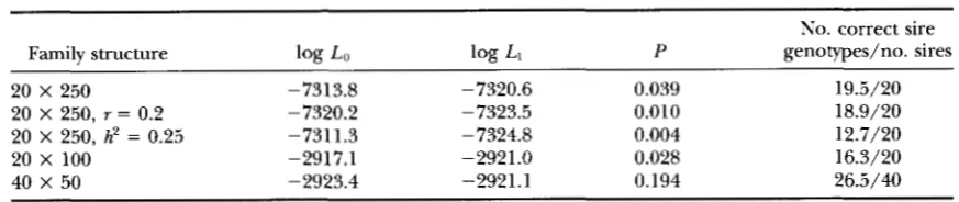
TABLE 5

Log likelihood ratio tests and proportion of correctly predicted genotypes

No. correct sire

Family structure log Lo log LI P genotypes/no. sires

20 X 250 -7313.8 -7320.6 0.039 19.5/20

20 X 250, r = 0.2 -7320.2 -7323.5 0.010 18.9/20

20 X 250, h2 = 0.25 -7311.3 -7324.8 0.004 12.7/20

20 x 100 -2917.1 -2921.0 0.028 16.3/20

40 X 50 -2923.4 -2921.1 0.194 26.5/40

Family structures are number of sires X number of progeny for sire. Replicate means of log likelihoods of

the full model (log Lo) and the reduced model with r = 0.5 (log L , ) , the probability, E‘, of the likelihood

ratio test for linkage being significant, and the proportion of sire genotypes ascertained correctly, for true

values of /I = 0.0, a = 0.5, d = 0.1, r = 0.1,

p

= 0.5, D = 1 and h‘ = 0, unless otherwise indicated.

765

experiment under these conditions. The likelihood ra-

tio test was significant at the 5% level for all combina-

tions, except for the simulations of 40 sires with 50

progeny per sire when it was significant at the 20%

level, on average. The corresponding power of these data sets, calculated using the approximate method of

WELLER et al. (1990) was >90% for all sets except the

40 X 50 data set.

The number of sire genotypes ascertained correctly,

averaged over replicates, are also given in Table 5 for

all parameter combinations and data set sizes simulated.

Prediction of sire genotype was 95% correct for the

data sets with 20 sires and 250 progeny per sire. As

expected, the proportion of correct assignments de-

creased with a reduction in the number of records. For the same number of records, the proportion of correct predictions was higher with more progeny per sire. This corresponds to the results given above with respect to standard errors of parameter estimates and likelihood ratio test probabilities. When adjustment for a poly- genic effect was included in the model, the number of correctly ascertained sire genotypes was much lower. Presumably, this is because a major source of informa- tion on sire genotype, the sire genotype mean, is re- moved by the adjustment. Thus, for the purposes of

sire genotype determination, it may be better to fit a

model without a polygenic effect in order to determine which sires have high probabilities of being heterozy- gous.

DISCUSSION

This study has demonstrated that it is feasible, both computationally and theoretically, to obtain unbiased estimates of the six parameters which describe a QTL

in a segregating outbred population. Attention was fo-

cused on the accuracy of the estimates of these parame- ters because this is crucial to the interpretation of the QTL’s characteristics and also how effectively the QTL is used in subsequent exploitative breeding programs. The development of a deterministic method based on infinite population sampling theory for predicting the lower bound standard errors of estimates was used to

demonstrate the various factors influencing accuracy. These factors are summarized and discussed below. However, the value of the deterministic technique re- quires discussion first, because it forms part of the basis for the conclusions drawn about those factors affecting accuracy.

Deterministic simulation: The deterministic method was based on infinite sampling in that it predicted num-

bers of observations with a given value based on the

density of the normal distribution and then used these “perfect” samples to perform a weighted analysis of the whole population. This implies that all the sampling variation in the data was due to random normal devia- tions within QTL genotypes within families. However, in finite populations, there is also expected to be a sampling effect on the numbers of animals that fall into each of the progeny marker-QTL genotype groups and also on the numbers of sires falling into each sire QTL genotype group. These multinomial sampling effects

were not accounted for in the calculation of the ex-

pected log likelihood (3) because the proportions in

each group were considered to be fixed as dictated by

the frequency parameters,

p

and t. While in data sets

of 5000 observations, this did not seem to be a problem,

in data sets of 2000, it is the most likely cause of the

clear underestimation of the predicted standard errors compared with the empirical standard errors, especially

when the families were smaller. The intermediate values

of

p

and t used in this study would have exacerbated

this sampling variation problem. Modification of (3)

to take these sampling effects into account could be

performed: to do so would involve calculating the ex-

pected log likelihood for values of n,c9 and sPh taken

over the whole range of the appropriate discrete

multinomial distribution, weighting accordingly by the multinomial probabilities of observing each value, and then summing to obtain an overall weighted likelihood. This would be considerably more complex than the method used here but deserves further investigation to see whether it accounts for the underestimation of the standard errors found using deterministic simulation.

rors, these estimates are considered to be useful for

predicting the minimum size of experiment required

to obtain a given level of accuracy of estimation of QTL

parameters. Also, the fact that they are lower bound

standard errors does not devalue the results concerning their behavior with respect to data structure, statistical

model used, and their relationship with each other.

This seems to be true because of the similar (though not always parallel) behavior of the empirical standard errors with changes in these conditions. Thus the con- clusions drawn below on the factors influencing accu- racy are considered valid.

Factors influencing accuracy of parameter estimates: The study identified five separate (though not indepen- dent) influences on standard errors of the parameters.

The first was the nature and magnitude of the parame-

ter itself. Recombination rate, r, was by far the most

inaccurate parameter and, even with 5000 observations, could not be estimated to an accuracy that was able

to exclude 0 recombination from the 95% confidence

interval. In this study, only a single marker adjacent to the QTL was considered. However, most other studies where accuracy has been examined have also consid-

ered two markers which bracket the QTL (KNOTT and

HALEY 1992a; VAN OOIJEN 1992; DARVASI et al. 1993) in

which case standard errors are reduced, though are still

large (0.05 -0.15) relative to the recombination fraction

itself. For example, DARVASI et al. (1993) estimated stan-

dard errors of 0.11 and 0.05 for a gene with an effect

of 0.5 standard deviations located at a recombination

distance of -0.1 from a single marker and bracket

markers space 20 cM apart, respectively, in a backcross

population of 1000 informative individuals. The closest

situation in this study is that for a gene effect of 0.5

standard deviations at a recombination distance of 0.1 in a population of 40 sires, only 20 of which were infor- mative, with 50 progeny each, where the standard error was 0.10. Thus the results presented here concur with

those of DARVASI et al. (1993) and VAN OOIJEN (1992)

that for most feasible experimental sizes, even when two markers bracket the QTL, the resolution of mapping a QTL is near the limit of the marker map itself (10-20

cM) and therefore other techniques need to be em-

ployed for fine mapping of the gene.

In contrast, reasonably accurate estimates of the gene

effects, a and d, can be obtained. Using the examples

above, the standard errors on a were found to be 0.06

and 0.05 in this and the study of DARVASI et al. (1993),

respectively. This is -10% of the parameter itself, which

is typical of the accuracy of many of the parameters used

in routine genetic prediction analyses. Several authors (e.g., SMITH and SIMPSON 1986) have pointed out the importance of the accuracy of QTL parameters in pre- dicting breeding values based on marker-QTL linkages, but most of the loss in prediction accuracy is likely to arise from inaccurate estimates of recombination rate rather than gene effect, as the consequences of infer-

ring a recombinant individual us. a nonrecombinant

individual are far greater than overestimating or under-

estimating by a small fraction the value of an individual. The influence of the magnitude of the gene effect on accuracy was not investigated directly. However, as the gene effect decreases, the power of the analysis also decreases because the between-marker contrast, which is the main source of information, is reduced also. This

reduction in power is similar to that caused by a de-

crease in experimental size; this was investigated in this study and shown to cause a decrease in accuracy.

The population mean and residual standard devia- tion were estimated relatively accurately as expected from the fact that all individuals in the data contribute information to these parameters, not just those from heterozygous sires. Though not investigated, the accu-

racy of the QTL allele frequency,

p,

is expected to de-

crease as the value of

p

tends towards extremes. This

is because the frequency of informative families will

decrease. It is expected that the accuracy of a, d and r

will also decrease for the same reason. It is worth noting

that accurate estimation of

p

is very important in some

situations because it determines how much scope for

genetic improvement there is to bring the favorable

QTL to fixation and therefore the value of a marker- assisted within-breed improvement program.

The second factor affecting accuracy of individual

parameters is the correlation with other parameters.

This study is the first to demonstrate that strong sam- pling correlations exist between some parameters. This result means that the accuracy of parameters cannot be considered in isolation, because correlations with other parameters cause a decrease in accuracy of the other

parameters. The implications are that if one parameter

is poorly estimated or biased for some reason, then correlated parameters will also be affected. The rela- tionships between parameters must be considered in the prediction of response to breeding programs that attempt to incorporate information on several parame- ters simultaneously.

The third factor affecting accuracy is total experimen-

tal size, and this influence is large. When experimental

size was increased by a factor of 2.5, the accuracy of

all parameters improved. It was found that parameters slightly increased in accuracy with an increase in family size or decrease in number of families when the total number of progeny is held constant, reflecting the im- portance of within-family information to estimate most parameters. These results are concomitant with a de- crease in power as family size decreases as also shown

by SOLLER and GENIZI (1978) and WELLER et al. (1990).

It is expected that the influence of family size on accu- racy would be more noticeable when the total experi-

mental size is smaller than that used in the present

study.

The fourth influence found to affect accuracy was the

Estimation of QTL Parameters 767

this can lead to overestimation of the QTL effect

(KNOTT et al. 1990; KNOTT and HALEY 199213). Here the adjustment used was to subtract the sire’s mean, which is similar to the “modal method” for adjusting for sire

effects used by HOESCHELE (1988) and LE ROY et al.

(1989) for segregation analyses to detect major genes without the aid of markers. In this study, it was shown to be an effective way of accounting for between-family variation without prior knowledge of polygenic herita- bility or simultaneous estimation of the between-family variation from the likelihood analysis. The latter ap-

proach was found to be necessary in the KNOTI and

H A L E Y study (1992b), which examined a full-sib design

in which family sizes were relatively small and therefore

family means were inaccurate. The effect of fitting a

polygenic model on parameter accuracy was to decrease

the accuracy of the parameters ( a and

d);

this contrib-

uted to the adjustment term because, in making the adjustment, much of the information on these parame-

ters is lost. Thus for the purposes of obtaining very

accurate estimates of the magnitude of gene effects, an alternative method for adjusting for between family

variation, such as that used by KNOTT and HALEY

(1992b) may be considered. Certainly, the effect of us- ing the polygenic model on the correlations between

parameters was to strengthen them, which is an undesir-

able consequence if several imperfectly estimated pa-

rameters are to be used simultaneosuly in breeding pro- grams.

The final influence on parameter accuracy examined in this study was that of assumed marker allele fre- quency. When wrong marker allele frequencies were used in the likelihood equation, the QTL was estimated to be larger and more distant from the marker than it really was. This problem is likely to be reduced as the heterozygosity of the marker increases because more progeny will have marker alleles that can be assigned to the sire and dam with certainty. Increased heterozy- gosity will certainly occur with the widespread transition

of use of diallelic markers such as RFLPs to polyallelic

markers such as microsatellites. The model presented here can be adjusted to account for multiple alleles by grouping the progeny into three marker genotype groups: one for those with the same genotype as the sire and two for those having either one of the sire’s alleles. In the current model, these groups would corre-

spond to the Mm, MM and m m groups and the frequen-

cies of the sire alleles in the dam population, t , and t . ~

would then replace t and (1 - t ) in the matrix C. One

problem that may arise is that with many alleles, marker frequencies estimated from the sample will be less accu- rate and wrongly assumed frequencies will influence the estimates, as shown in this study. One way to avoid this is to only use data from animals that have been

unambiguously assigned a paternal and maternal allele,

although this would result in loss of information and hence loss of accuracy of the estimates. Sensitivity to

assumptions about marker allele frequency is a well

known problem in linkage analysis of discrete traits.

So far, the information yielded by the likelihood on

the QTL parameters has been discussed. However, the likelihood also yielded information on the genotypes of the sires and was found to very accurately predict the sire’s genotype when the number of progeny was

>loo.

This information is of great practical impor-

tance when the ultimate goal of the experiment is to select sires carrying favorable QTL alleles for commer- cial breeding via marker-assisted selection (WELLER

and FERNANDO 1991). This prediction method may

also be used to eliminate the uninformative QTL ho- mozygous sires at the early stage of a QTL mapping experiment, although where there are multiple QTL

to detect, there will be few sires that are homozygous

for all QTL and therefore able to be discarded. The confidence with which sires can be classified into QTL genotypes needs further investigation, especially when there are many possible QTL genotypes, in which case

the test of one genotype us. the rest requires some

knowledge of the properties of this multiple hypothe- sis test statistic.

The implications of violations of the assumptions of the model will be briefly considered. The model

assumed underlying normality and equal variance

among QTL genotypes and that the progeny with rec- ords were a random sample of the sire’s progeny. Skew- ness and kurtosis may lead to false conclusions about

major gene effects (GO et al. 1978). If there is skewness,

the analysis can be performed on transformed data,

as suggested by WELLER (1987), although overcorrec-

tion of the skewness can remove some of the informz- tion on the QTL from the mixture of distributions.

DARVASI (1990) found that estimation of QTL parame-

ters by ML under the assumption of equal genotype

variance resulted in accurate estimates for genotype means even if this assumption was incorrect, provided that the actual variances were not radically different. If recorded progeny are a selected sample, estimates

of QTL effects will be severely biased (MACKINNON and

GEORGES 1992). Incorporation of a truncation param-

eter in the likelihood model presented here may be

one way of accounting for the effects of selection. The

degree of selection would, however, have to be known from an independent analysis.

Conclusions: The study showed both theoretically and empirically that unbiased estimates of the six pa-

rameters that determine a QTL effect in the half-sib

design are able to be estimated by maximum likelihood

methodology via linkage to a genetic markers. All pa-

rameters except for recombination frequency and the QTL’s dominance effect are accurately estimated rela- tive to the size of the parameter itself when there are several thousand progeny records. Further improve- ments in accuracy may be obtained by including other

markers in the model that reduce the background varia-

tion ( JANSEN 1993; ZENC 1994). Parameter estimates