ABSTRACT
YOO, WILLIAM WEIMIN. Sup-norm Posterior Convergence Rates for Regression Models with Application to Estimating the Location of Function Maximum. (Under the direction of Subhashis Ghoshal.)
In the setting of nonparametric multivariate regression with unknown error variance σ2, we propose a Bayesian method to estimate the regression function f and its characteristics, with particular interest in estimating its mixed partial derivatives, location of function maximumµ
and its value maximumM. Our prior consists of representingf using tensor-product B-splines with normal basis coefficients, where σ2 is either estimated using empirical Bayes or endowed with an inverse-gamma prior. The frequentist properties of the resulting posterior distributions and credible sets are studied extensively. In particular, we establish pointwise,L2-and sup-norm posterior convergence rates for f and its mixed partial derivatives, and show that they coin-cide with the minimax rates. Also, pointwise, L2-and sup-norm credible sets are constructed to reflect their estimation uncertainties. Under appropriate conditions, we show that they have guaranteed frequentist coverage with optimal size up to a logarithmic factor. We extent our results on posterior convergence rates and credible sets to anisotropic f, such that f has dif-ferent smoothness in each dimension. In addition, we introduce new results on tensor-product B-splines.
We derive an inequality that relates sup-norm distance of partial derivatives of f with Euclidean distance ofµ, and also prove a similar inequality betweenf andM. Hence, posterior convergence rates and credible sets established forf and its mixed partial derivatives translate directly toµandM. Moreover, we propose a two-stage Bayesian procedure to estimate these two quantities. In the first stage, we endow f with the tensor-product B-splines prior as described. We then construct credible region forµbased on the posterior distributions off and its mixed partial derivatives. We sample from this region and represent f as a multivariate polynomial with normal coefficients. The corresponding induced posterior distributions ofµandM will have improved posterior convergence rates. In particular, for α-smooth f, the optimal single-stage posterior convergence rates (logn/n)(α−1)/(2α+d) and (logn/n)α/(2α+d) forµand M improve to
©Copyright 2014 by William Weimin Yoo
Sup-norm Posterior Convergence Rates for Regression Models with Application to Estimating the Location of Function Maximum
by
William Weimin Yoo
A dissertation submitted to the Graduate Faculty of North Carolina State University
in partial fulfillment of the requirements for the Degree of
Doctor of Philosophy
Statistics
Raleigh, North Carolina
2014
APPROVED BY:
Brian Reich Donald Martin
Arnab Maity Subhashis Ghoshal
DEDICATION
BIOGRAPHY
The author was born in Georgetown, Penang, Malaysia on 3rd February, 1986. After finishing high school, he enrolled in the American Degree Transfer program to pursue a Bachelor’s degree in Actuarial Science. As a result, he spent two years at INTI International College, Nilai, and two years abroad at Drake University, Des Moines, Iowa. After graduating, he worked briefly as an Actuarial Executive at Allianz Life Insurance Malaysia. While trying to introduce stochas-tic models for future reserve computation, he realized that his current statisstochas-tical knowledge is limited and needed more advanced methods. Therefore, he decided to do a Master’s in statis-tics at the University of Waterloo, Canada. His passion for research and his inclination toward academia lead him to further pursue a PhD in statistics at the North Carolina State University in the U.S.A.
ACKNOWLEDGEMENTS
TABLE OF CONTENTS
LIST OF TABLES . . . vii
LIST OF FIGURES . . . .viii
Chapter 1 Introduction . . . 1
1.1 Bayesian nonparametrics . . . 1
1.2 Bayesian nonparametric regression . . . 2
1.3 Priors on regression functions . . . 4
1.3.1 Gaussian process . . . 4
1.3.2 Random series . . . 5
1.4 Consistency and convergence rates . . . 6
1.5 Coverage and credible region . . . 9
1.6 Research questions and our contributions . . . 10
1.6.1 Sup-norm convergence rates forf and its mixed partial derivatives . . . . 11
1.6.2 L∞-credible sets for f and its mixed partial derivatives . . . 12
1.6.3 Bayesian estimation of location of maximumµand maximum value M . 12 1.7 Notations and preliminaries . . . 13
1.8 Chapter organization . . . 16
1.8.1 Chapter 2: Sup-norm posterior convergence rate for univariate regression 16 1.8.2 Chapter 3: Sup-norm posterior convergence rate for multivariate regression 16 1.8.3 Chapter 4: Bayesian procedure for estimating location of maximum . . . . 17
1.8.4 Chapter 5: Two-stage Bayesian estimation ofµand M . . . 17
1.8.5 Appendices . . . 17
Chapter 2 Sup-norm posterior convergence rate for univariate regression . 18 2.1 Introduction . . . 18
2.2 Prior and posterior conjugacy . . . 20
2.3 Posterior convergence rates for f . . . 27
2.4 Posterior convergence rates for derivatives . . . 32
2.5 Credible sets for f and its derivatives . . . 37
2.6 Simulation . . . 46
Chapter 3 Sup-norm posterior convergence rate for multivariate regression 57 3.1 Introduction . . . 57
3.2 Prior and posterior conjugacy . . . 59
3.3 Posterior convergence rates for f . . . 67
3.4 Posterior convergence rates for mixed partial derivatives . . . 72
3.5 Extension to anisotropic H¨older space . . . 79
3.5.1 Anisotropic posterior convergence rates for mixed partial derivatives . . . 83
3.6 Credible sets for f and its mixed partial derivatives . . . 85
Chapter 4 Bayesian procedure for estimating location of maximum . . . 97
4.2 Credible regions forµand M . . . 102
Chapter 5 Two-stage Bayesian estimation of µand M . . . .109
5.1 Introduction . . . 109
5.2 Two-stage Bayesian procedure . . . 109
5.3 Simulation . . . 124
References. . . .131
Appendices . . . .139
Appendix A New Results on Univariate B-splines . . . 140
Appendix B New Results on Tensor-product B-splines . . . 143
Appendix C Sub-Gaussian Inequalities . . . 152
LIST OF TABLES
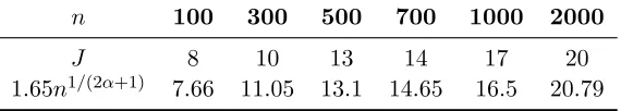
Table 2.1 OptimalJ by CV (Bayes) vs. ComputedJ based on asymptotic formula with
LIST OF FIGURES
Figure 1.1 The red dot is the point of global maximum, we are interested in determining the location of this point in thex, y plane below and its maximum value. . . 4 Figure 1.2 Sample paths generated from a Brownian motion, each of this path is a
continuous function inR. . . 5 Figure 1.3 The figure on the left is the truef, while on the right is the posterior mean
of f using bivariate cubic B-splines random series. . . 6 Figure 1.4 Schematic diagrams: testing problem in (1.6) on the left while the right shows
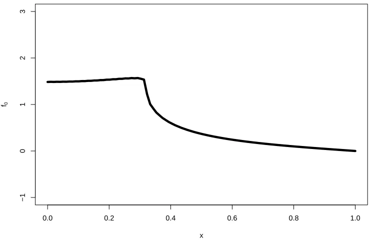
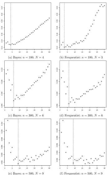
the number of balls needed to cover Θn (covering number). . . 8 Figure 2.1 A set of 10 cubic (q= 4) B-splines. . . 20 Figure 2.2 A plot off0, note the distinguishing bump nearx= 0.3 . . . 47 Figure 2.3 CV mean square error againstN number of interior knots. Vertical dash lines
indicate optimal N. . . 51 Figure 2.4 CV mean square error againstN number of interior knots. Vertical dash lines
indicate optimal N. . . 52 Figure 2.5 Pointwise coverage probabilities for credible and confidence intervals. . . 53 Figure 2.6 Pointwise coverage probabilities for credible and confidence intervals. . . 54 Figure 2.7 Red: posterior mean (left) and fb(right), Black: true function, Blue dash:
95%L∞-credible (left) and confidence (right) bands. . . 55 Figure 2.8 Red: posterior mean (left) and fb(right), Black: true function, Blue dash:
95%L∞-credible (left) and confidence (right) bands. . . 56
Figure 3.1 A set of 100 bivariate cubic B-splines. To show the inner structure, only the last 50 is plotted. . . 59
Figure 4.1 A function that has no well-separated maximum. This function `(θ|·) has global maximum at θ0, but the horizontal asymptote is approaching this maximum as well. . . 100
Figure 5.1 A plot off0, with the true maximum indicated by the red dot. . . 125 Figure 5.2 A plot off0, with gray points as the first stage 625 observations. . . 126 Figure 5.3 Posterior mean based on bivariate B-spline prior, the location corresponding
to red dot is µbn, and grey points are the 670 second stage samples. . . 126
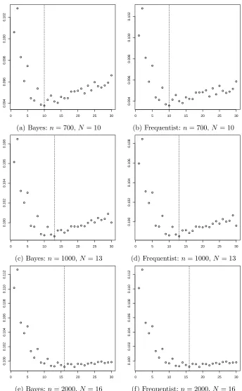
Figure 5.4 The second stage posterior density for µ. . . 127 Figure 5.5 Box plots of 1000 computed kµe2nd −µ0k, where µe2nd is the second stage
Bayesian (left) or frequentist (right) estimator ofµ0for eachδ = (0.01, . . . ,0.2).128 Figure 5.6 CV mean square error againstN number of interior knots at each dimension.
Vertical dash lines indicate optimalN. . . 128 Figure 5.7 L2-norms of the difference between Bayesian or frequentist estimator with
Chapter 1
Introduction
1.1
Bayesian nonparametrics
Bayesian nonparametrics is the application of Bayesian principles to nonparametric models for parameter estimation and inference. These models contain infinite-dimensional parameters and do not assume specific functional form for the true distribution. Bayesian inference on these models consists of two main steps: specifying prior distribution on these infinite-dimensional parameters, and combine the prior with the likelihood through Bayes formula to produce the corresponding posterior distribution.
Unlike parametric models, which have overly restrictive and often unjustifiable assumptions on the data generating mechanism, these models are flexible and can be applied to a wide va-riety of statistical problems. A canonical example is density estimation where the parameter is the density function itself. Another example, which will be the main focus of this dissertation is regression, where the regression function is unknown and assumed to belong to a function class. Additional examples include estimation of spectral density in time series, hazard rate function in survival analysis, transition density of Markov chain, nonparametric hypothesis tests and others. The Bayesian paradigm provides a unified and consistent framework for parameter esti-mation and inference, since all quantities of interest such as point estimator and credible regions can be derived solely from the posterior distribution. In addition, the development of Markov Chain Monte Carlo (MCMC) sampling methodologies has provided a tremendous boost to the use of Bayesian nonparametrics in practical applications. For example in genetics, machine learning, neuroscience, engineering and many more.
poses unique conceptual and technical challenges. Natural choices of prior for certain statis-tical problem might lead to an inconsistent posteriors, i.e., a posterior distribution that does not concentrate at the true value of the parameter asymptotically. The inclusion of the true parameter in a prior’s topological support does not by itself guarantee posterior consistency. This stems from the fact that it is possible to construct priors on infinite-dimensional spaces that will not be overwhelmed by the data even if we had indefinitely large sample sizes.
To avoid these difficulties, a list of default priors are introduced and catalogued for different problems. Such priors are constructed through some automatic mechanism and their mass is spread across the parameter space. Also, they are impartial with respect to any particular pa-rameter, and they have low information content compared to the data. They are analogues to improper priors in parametric Bayesian inference, but these default priors are invariantly proper on infinite-dimensional spaces. Examples of default priors include Dirichlet process (Ferguson, 1973), Dirichlet mixtures (Ferguson, 1983, Lo, 1984), Gaussian process (Leonard, 1978, Lenk, 1988) and random series.
Sampling from the posterior distribution of infinite-dimensional parameters requires inno-vative and novel sampling strategies. The basic idea is to decompose the posterior into more elementary components, and reduce the problem into sampling from these finite-dimensional pieces. Often, the sampling problem is cast into a hierarchical framework by introducing latent variables. Examples include Gibbs sampling based on P´olya urn (MacEachern, 1994, Escobar and West, 1995) with its variants such as stick breaking Gibbs (Ishwaran and James, 2001) and no-gaps algorithm (MacEachern and M¨uller, 1998), Metropolis-Hastings with Gibbs sam-pling (Neal, 2000), slice samsam-pling (Walker, 2007), non-MCMC samsam-pling based on random series (Shen and Ghosal, 2014), variational methods (Blei and Jordan, 2006), and direct sampling if the posterior distribution has explicit expression due to conjugacy.
In the next section, we discuss Bayesian nonparametric regression, which is one of the main applications of Bayesian nonparametrics.
1.2
Bayesian nonparametric regression
The Bayesian nonparametric regression problem is as follows: suppose we have noisy observa-tions from some unknown function f :Rd→Rsuch that
where the covariatesXi ∈U withU some bounded open set inRd, andεi are independent and identically distributed (i.i.d.) errors. Our aim is to estimate f and perhaps some of its other characteristics. Since f is unknown, we will typically assume that f belongs to some known function space F. A Bayesian will then put a prior on f, compute its posterior, use the pos-terior mean as estimate forf and quantifies its uncertainty by constructing credible sets forf
based on posterior variance.
There is a close connection between regression with spline theory since f can be modeled as splines in some applications. In this framework, Kimeldorf and Wahba (1970) and Wahba (1978) appear to be the first to use Gaussian process as prior for f, where they used what is called the integrated Brownian motion polynomially released at zero. Cox (1993) expanded f
using random series with eigenfunctions as basis. de Jonge and van Zanten (2012) represented
f using tensor-product B-splines and studied its asymptotic properties.
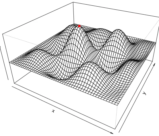
Certain characteristics off are also of interest. For example the derivatives of the regression function assuming that the function is smooth enough. The location of the function maximum and its maximum value are useful characteristics that we will fully investigate in this dissertation (see Figure 1.1). Other characteristics include location of change-points or jump discontinuities and estimating the inverse of a regression function evaluated at a point in the function’s range.
The regression function and its associated characteristics can be estimated in one or multi-stages. In this context, single-stage estimation means we use a fixed design to collect all samples for estimation in one go. For multi-stage estimation, we employ instead sequential design to collect samples, i.e., one collects samples based on information gathered from previous samples, and estimation is conducted through stages. It has been proven by many research papers that multi-stage estimation improves the accuracy of the estimate, and it is possible to construct estimators in sequential designs that have faster convergence rates than the minimax rates for single-stage procedures. Examples in the literature include two-stage estimation of location of function maximum (Belitser et al., 2012), change-points (Lan et al., 2009) and inverse regression (Tang et al., 2011).
x
y ●
Figure 1.1: The red dot is the point of global maximum, we are interested in determining the location of this point in the x, y plane below and its maximum value.
1.3
Priors on regression functions
1.3.1 Gaussian process
Let X ={X(t) :t∈U} be a stochastic process indexed by U ⊆Rd. Define its mean function as E[X(t)] =µ(t) and covariance function as Cov[X(t), X(s)] =V(t,s) for any t,s∈Rd. We sayX is a Gaussian process if for anynfinite collection of points t1, . . . ,tn,
[X(t1), . . . , X(tn)]∼Nn(µ,V), (1.2) whereµ= (µ(t1), . . . , µ(tn))T andV is the Gram matrix of the covariance functionV(·,·), i.e.,
vij =V(ti,tj) for 1≤i, j≤n.
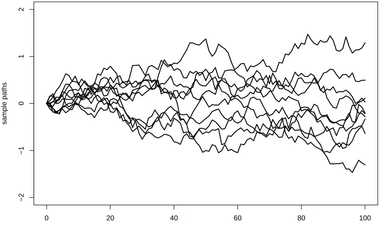
and van Zanten, 2008a). Specific instances of Gaussian processes include the Brownian mo-tion or Wiener process (Figure 1.2), integrated Brownian momo-tion, fracmo-tional Brownian momo-tion, Riemann-Liouville process (see Section 4.2 of van der Vaart and van Zanten, 2008b).
0 20 40 60 80 100
−2
−1
0
1
2
time
sample paths
Figure 1.2: Sample paths generated from a Brownian motion, each of this path is a continuous function inR.
1.3.2 Random series
Let f :R→ R be the regression function in (1.1) such that f ∈ F. Suppose {φj :j ≥ 1} is a set of basis forF, then we can representf truncated at level J as
f(x) = J
X
j=1
θjφj(x). (1.3)
The above series representation is a random function and hence its name random series. Depend-ing on the underlyDepend-ing function spaceF, commonly used basis functions include the polynomials, Fourier basis, B-splines and wavelets. Prior elicitation can be accomplished by putting sepa-rate independent priors on (θ1, . . . , θJ)T and J respectively. This will then induce a prior on
x
y
x
y
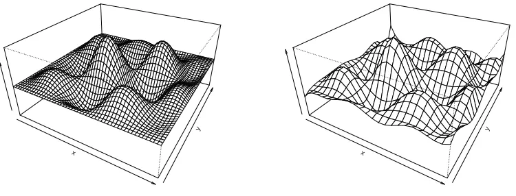
Figure 1.3: The figure on the left is the true f, while on the right is the posterior mean of f
using bivariate cubic B-splines random series.
be represented as a infinite random series with normal coefficients, and the eigenfunctions of its covariance function as basis. Random series is a powerful tool in Bayesian nonparametrics. With appropriate choices of basis and priors on the coefficients, random series can approximate a wide variety of functions well (see Figure 1.3).
1.4
Consistency and convergence rates
Due to the sheer size of an infinite-dimensional parameter space, there is no guarantee that the posterior distribution will converge to the point mass of the truth, even if the truth is contained in the support of the prior. This property, which we call posterior consistency holds in finite-dimensional parametric models under relatively mild conditions, but a much more in-volved analysis is needed to establish consistency in nonparametric models. Freedman (1963) constructed an example using geometric distribution showing posterior inconsistency. Other examples can be found in Diaconis and Freedman (1986) for location models and de Blasi et al. (2013) for Gibbs-type priors. The celebrated Schwartz (1965) paper introduced the concept of using Kullback-Leibler neighborhoods and test with exponentially small errors to prove consis-tency for dominated statistical models. Extensions of Schwartz’s result were provided by Barron et al. (1999) and Ghosal et al. (1999).
Since the definitions given below apply to more general parameter spaces, we will tem-porarily leave the regression framework. Let Θ be the parameter space endowed with a met-ric d and a Borel sigma-field B. Let θ0 ∈ Θ be the true parameter. Suppose we observed
let Pθ(n)
0 be the corresponding true joint distribution and define X
(n) to be the sample space of
X. Note we do not assume independence or i.i.d. structure of the observations. Given a prior Π on the Borel sets of Θ, let Π(·|X) denote the corresponding posterior. We say that the posterior distribution Π(·|X) is consistent atθ0 if for any >0,
Π(θ:d(θ, θ0)> |X)→0 (1.4)
in Pθ(n)
0 -probability as n → ∞. Consistency is a frequentist concept. But applying it in the
Bayesian context means that as we collect more and more samples, the posterior distribution will converge to the point mass of θ0. Another implication of consistency is that with large enough samples, posterior distributions computed using different priors will agree (their dis-tances in weak topology will go to zero). Hence Bayesians with different prior beliefs will have their opinions merged, and will ultimately reach a consensus iff consistency holds.
We can take this concept one step further by asking how fastcan go to 0 withnmaintaining the property that the posterior probability in (1.4) goes to zero. This rate of convergence can be succinctly described as follows: given a positive sequence n such that n →0, we say that posterior distribution Π(·|X) converges to θ0 at the rate n with respect to the metric dif for any sequence Mn→ ∞,
Π(θ:d(θ, θ0)> Mnn|X)→0 (1.5) in Pθ(n)
0 -probability as n → ∞. We are naturally interested in the fastest rate possible, i.e.,
smallest n. Often the optimal rate will be equal to the minimax estimation rate in the fre-quentist sense up to a constant or logarithm factor. In our case, Θ is the function space F
with true function f0. We will study supremum norm (sup-norm for short) convergence rates of f ∈ F and its derivatives, where the metric used is the function supremum norm, i.e.,
d(f, f0) =kf −f0k∞= supx∈U|f(x)−f0(x)|. Note that estimating the derivatives off can be viewed as an inverse problem.
If we had analytic expression for the posterior through conjugacy, then (1.5) can be estab-lished by Markov’s inequality. If not, then more elaborate theory is needed. In this case, there are usually four conditions that we need to verify depending on the dependence structure of
𝑷𝜽
𝟎
(𝒏)
𝑷𝜽(𝒏)𝟏
> 𝝐
radius 𝝃𝝐
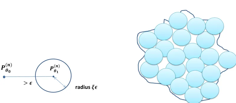
Figure 1.4: Schematic diagrams: testing problem in (1.6) on the left while the right shows the number of balls needed to cover Θn (covering number).
testing problem. Let ξ, n > 0 and some θ1 ∈ Θ. Suppose X ∼ P for some joint probability distributionP and we wish to test the following (see left panel of Figure 1.4):
1.5
Coverage and credible region
Given parameter space Θ. Let θ0 ∈Θ be the true parameter. We say that a subsetC(X) of Θ is a 1−γ credible region or set if the posterior mass of C(X) is 1−γ forγ ∈[0,1]. That is,
Π(θ:θ∈C(X)|X) = 1−γ. (1.7)
Credible regions are used to quantify the uncertainty of estimatingθ, with the posterior spread indicating the margin of error in estimation. Unlike frequentist’s confidence regions, (1.7) is a true probability statement and we can say the posterior probability of θ falling in C(X) is 1−γ. We note that C(X) depends on the data X. In parametric Bayesian inference, various criteria were proposed as to what constitute the best 1−γ credible region, and methods were developed to construct them. For example, constructing the highest posterior density (HPD) credible region, where we try to find the smallest C(X) region that satisfies (1.7). In finite-dimensional setting, the credible region constructed will have the right asymptotic frequentist coverage in most cases, i.e., as n→ ∞,
Pθ(n)
0 (θ0 ∈C(X)) = 1−γ. (1.8)
However, this is no longer true for credible region constructed for infinite-dimensional parame-ters. Using the Gaussian white noise model, Cox (1993) concluded that Bayesian credible sets at any level have frequentist coverage zero for almost all true θ0. This disparaging conclusion was furthered enforced by Freedman (1999) and he provided instances of credible sets with asymptotically zero or sub-optimal coverage. It may be noted that their formulation consists of drawing true function (equivalently sequences) from the prior itself, and failure is shown in the almost sure sense with respect to the prior. The main cause of this is that in finite-dimensional problems, the Bernstein-von Mises theorem holds. That is, the posterior distribution converges to a normal distribution centered at the maximum likelihood estimate, with the inverse Fisher information as its variance. Hence, if the sample size is large enough, credible sets will behave like confidence regions and they will have asymptotically the right coverage. However, there is often no Bernstein-von Mises theorem for nonparametric models and credible sets constructed for these models are not guaranteed to have the right coverage. On the other hand, Leahu (2011) and Castillo and Nickl (2013) showed that if the parameter space is extended beyond`2 sequence space, and normal priors with large variances are used for each component, then the credible regions do possess adequate frequentist coverage.
un-dersmoothing the prior, we can construct conservative credible sets with coverage tending to 1. They then applied their findings to the problem of heat equation in Knapik et al. (2013). On the other hand, Castillo and Nickl (2013) extended Leahu (2011) work beyond conjugate priors and obtained parametric posterior convergence rates under norms weaker than the `2-norm, called negative Sobolev norms. Assuming a weak Bernstein-von Mises phenomenon, Castillo and Nickl (2013) constructed credible sets with right frequentist coverage for white noise mod-els. They also showed that Bernstein-von Mises result holds for the negative Sobolev norm under appropriate condition on the prior. Recent research considers the issue of constructing adaptive credible sets, where these sets have guaranteed frequentist coverage with radius that adapts to the unknown regularity of θ0, or function smoothness if Θ is a function space (see Hoffman et al., 2013 and Szabo et al., 2014 for more details).
Motivated by the previous discussion, we will consider a reformulation of the Bayesian credibility problem. For a given sequence Ln→ ∞, our aim is to find a subsetC(X)⊆Θ with the following properties, uniformly forθ0 ∈D whereDis a ball in Θ:
1. Π(θ∈C(X)|X) = 1−ωn inPθ(n)0 -probability, 2. Pθ(n)
0 (θ0 ∈C(X))→1,
3. diam(C(X)) =OP(n) θ0
(Lnn),
where n is the minimax convergence rate for θ. The first condition creates a 1−ωn credible region, where ωn∈[0,1] can be fixed or a sequence tending to 0. If ωn is a constant, then the second condition holds if we inflate the radius of C(X) by some factor, or we use a prior onθ
that is less regular than the true regularity ofθ0 (undersmoothing if Θ is a function space with function smoothness as a measure of regularity). The second condition says that the frequentist coverage under the true distribution of the credible region goes to one asymptotically. The last condition limits the size of the constructed credible region by forcing it to have diameter at mostLnn.
1.6
Research questions and our contributions
1.6.1 Sup-norm convergence rates for f and its mixed partial derivatives Convergence rates underL2-norm and Hellinger distance were the first to be derived and stud-ied, and the corresponding theory is well established. However, theory for convergence rates in stronger norms such as the supremum norm is limited and has only caught attention in recent years. In addition, there is an inequality relating the sup-norm distance of partial derivatives of f and the Euclidean distance of µ. Also, similar inequality holds between f and M. This implies that the posteriors off and its partial derivatives induce the same sup-norm rate on the posteriors ofM and µ. Therefore, these two factors motivate the study of sup-norm posterior convergence rates for f and its mixed partial derivatives.
The first paper to tackle this problem was Gin´e and Nickl (2011), where they derived rates inLr-metrics for all 1≤r≤ ∞, and they constructed new tests with exponentially small error probabilities based on Talagrand’s inequality to handle L∞-convergence. However their rates are sub-optimal for r > 2, and they showed using a white noise model that optimal rate is achievable for conjugate priors with diagonal structure. Castillo (2014) introduced techniques based on semiparametric Bernstein-von Misses type results to obtain optimal sup-norm rates, for the white noise model and density estimation using priors based on wavelet series. He split the sup-norm distance into smaller components consisting of semiparametric functionals, and the corresponding influence function is estimated using various uniform approximation schemes. Hoffman et al. (2013) derived optimal adaptive sup-norm convergence rate for white noise model using spike and slab priors. They then generalized their result by introducing sieve priors that achieve the same adaptive sup-norm rate. For density estimation, Scricciolo (2014) employed Gaussian kernel mixtures by endowing the mixing distribution with a Pitman-Yor or normal-ized inverse Gaussian process. She obtained adaptive posterior convergence rates in Lr-metric for 1≤r≤ ∞.
Most of the papers on sup-norm convergence rate focus on density estimation and white noise model with known error variance, and contain only brief mentions of nonparametric re-gression. Also, all papers considered univariate models. Most papers use random series prior with wavelets as basis. In this dissertation, we will derive sup-norm convergence rates for multi-variate nonparametric regression in the setting of (1.1). Instead of using wavelets, we represent
implicitly as inverse problems in white noise models. Moreover, we allow function to have dif-ferent smoothness in difdif-ferent dimensions, which is a useful generalization. In addition, we let
σ be unknown, thus making the results more relevant for practical applications. The sup-norm convergence rates under our proposed prior coincide with the minimax rates of estimating a function and its mixed partial derivatives.
1.6.2 L∞-credible sets for f and its mixed partial derivatives
The issue of constructing nonparametric confidence set has been studied by many authors. In particular, Juditsky and Lambert-Lacroix (2003), Robins and van der Vaart (2006) and Cai and Low (2006) showed that it is impossible to construct adaptive confidence sets that are simul-taneously honest, and have radius that adapt to the underlying function smoothness. Bayesian analog of a confidence set is given by a credible region in which has a guaranteed posterior probability. Construction of credible sets in the context of function estimation is a challeng-ing problem, since optimal smoothchalleng-ing typically makes the order of the bias and variability the same. They are typically easy to obtain numerically from posterior sampling. Hence it is of considerable interest to know that a credible region possesses asymptotically correct frequentist coverage.
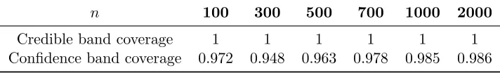
The issue of constructing credible sets for nonparametric models, and evaluating their per-formance has received very little attention in the Bayesian nonparametrics literature, with the main references mentioned in Section 1.5. Most of the credible sets for f in these papers are sets in sequence `2-or function L2-Hilbert spaces, while sets in L∞-Banach space are not well understood. Using our tensor-product B-spline prior, we propose methods to construct L ∞-credible sets for f and its mixed partial derivatives that satisfy the criteria listed in Section 1.5. In addition, we will also construct pointwise credible intervals forf(x) at any x∈(0,1)d and L2-credible sets for f. Under appropriate conditions, all pointwise, L2-and L∞-credible sets are shown to have frequentist coverage tending to 1 asymptotically with optimal size up to a logarithmic factor. Moreover, we carried out extensive simulations to compare finite sample performance of our pointwise credible intervals and credible bands with pointwise confidence intervals and confidence bands proposed by Zhou et al. (1998).
Kiefer and Wolfowitz (1952) proposed a Robbins-Monro type algorithm using sequential sam-pling to estimateµin one-dimension. Blum (1954) extended their method to higher dimensions. Mokkadem and Pelletier (2007) provided a method to simultaneously estimate µ and M in a sequential design setting. Belitser et al. (2012) proposed a two-stage procedure for estimation of these two quantities and studied its asymptotic properties.
However, the papers described above used frequentist methods in estimating µ and M, and a Bayesian equivalent is lacking. Therefore, we will study this problem in a Bayesian setting. Inspired by Belitser et al. (2012), we will propose a Bayesian two-stage procedure to estimate µ and M. We study its asymptotic properties and investigate its finite sample performance through a series of simulations. In particular, we show that our proposed Bayesian two-stage procedure performs better in terms of mean square error than other common single-stage methods, and is as good as the frequentist two-single-stage procedure proposed in Belitser et al. (2012). We hope that this dissertation is a first step towards providing a Bayesian solution to this problem.
1.7
Notations and preliminaries
We describe notations and technical definitions used throughout this dissertation. All asymp-totic relations and symbols described below refer to the regimen→ ∞. Given two numerical se-quencesanandbn,an=O(bn) oran.bnmeansan/bnis bounded, whilean=o(bn) oranbn means an/bn →0. Also, an bn means an=O(bn) andbn=O(an). Furthermore,an ∼bn is
an/bn → 1. For stochastic sequences Xn, Xn = OP(an) means that P(|Xn| ≤ Can) → 1 for some constant C >0, while Xn =oP(an) meansP(|Xn| ≤) →1,∀ >0. LetN ={1,2, . . .} be the set of natural numbers and N0=N∪ {0}.
Vectors are represented by bold symbols and can be upper or lower case English or Greek letters. All vectors are in column format and the corresponding non-bold letters with subscript denoting the components, i.e., for x,xi ∈ Rd, x = (x1, . . . , xd)T and xi = (xi1, . . . , xid)T respectively. Letkxkp be the vectorp-norm, i.e.,kxkp = (Pdk=1|xk|p)1/p. Ifp= 2, we suppress the subscript and simply write kxk to be the usual Euclidean norm. Given another vector y
of the same dimension, we write x ≤ y if xk ≤yk, k = 1, . . . , d. Matrices are written in bold and only upper case English letters are used to denote them. For a given symmetric matrix A
of dimension m×m, we denote its (i, j)th element by aij. Let λmin(A) and λmax(A) denote the smallest and largest eigenvalues respectively. Denote Λ(A) to be the set of eigenvalues of
(2,2) and (∞,∞) norms are defined as
kAk(2,2) =
q
λmax(ATA) =|λmax(A)|, kAk(∞,∞)= max
1≤i≤m m
X
j=1
|aij|= max 1≤j≤m
m
X
i=1
|aij|,
where they are the usual operator norms if we view A as a continuous linear operator on (Rm,k · k) and (Rm,k · k∞) respectively. In addition, define the matrix max-norm askAk∞= max1≤i,j≤m|aij|. Then the max-norm, (2,2) and (∞,∞) matrix norms are related by kAk∞≤
kAk(2,2) ≤ kAk(∞,∞). With another symmetric and square matrixB of the same size, A≤B
means B−A is non-negative definite and A <B meansB −A is positive definite. We say thatAis aq-banded matrix ifaij = 0 for|i−j|> q. Also, we denoteImas the m×midentity matrix and 1d as the vector of ones with dimension d. We define diag(a1, . . . , am) to be the diagonal matrix with diagonal elements (a1, . . . , am)T.
For f :U → R on some bounded open set U ⊆Rd, let kfk
p be the Lp-norm, i.e., kfkp = (R |f|pdν)1/pfor some sigma-finite measureν. If the integrating measure needs to be emphasized, we write kfkp,G = (
R
|f|pdG)1/p. If p = ∞, kfk
∞ = supx∈U|f(x)|. For a real-valued random variable X and a function ψ : [0,∞) → [0,∞), which is nondecreasing, convex andψ(0) = 0, we define the Orlicz norm ofX as
kXkψ = inf
C >0 : E
ψ
|X|
C
≤1
.
We note that if ψ(x) =xp for p≥1, then kXkψ =kXkp. We will mainly use the exponential Orlicz norm, ψp(x) =ex
p
−1 for p= 2 throughout this dissertation. ForI ⊂U, let f|I denote the restriction off onto I such thatf(x) =f|I(x) forx∈I. Furthermore, let1U(x) be the in-dicator function onU such that1U(x) = 1 forx∈U and 0 otherwise. Define an Euclidean ball of centerawith radiusRinU to beB(a, R) ={y:ky−ak ≤R}. Forδ >0, letN(δ, U,k · k) be the covering number of U, and is defined as the minimum number of Euclidean balls of radius
δ needed such that their union contains U. Let diam(U) = supx,y∈Ukx−yk be the diameter ofU. We defineUdto be the d-fold Cartesian product ofU, and|U|to be the cardinality ofU.
For multi-index i= (i1, . . . , id)T ∈Nd0 and a vectorx∈Rd, define
|i|= d
X
k=1
ik, i! = d
Y
k=1
ik, xi= d
Y
k=1
xik
We denotePn= span{xi :|i| ≤n}to be the space of multivariate polynomials of ordern. Here,
span{a1, . . . , ad} means the set of all possible linear combinations of a1, . . . , ad. Furthermore, fork, r∈N0 andd∈N, we define
Ik={i∈Nd0 :i1+. . .+id=k}, I(r) = r
[
k=0 Ik.
Here we enumerate I(r) as I0∪I1 ∪. . .∪Ir. Also, the elements within each Ik are arranged lexicographically. Fori6=j,Ii∩Ij =∅. The cardinality ofIk and I(r) are given by
|Ik|=
d+k−1
d−1
, |I(r)|= r
X
k=0
|Ik|= r
X
k=0
d+k−1
d−1
.
Let Hf(x0) be the Hessian matrix of f at x0 ∈Rd, whose (i, j)th entry evaluated at x=x0 is∂2f(x)/∂xi∂xj|x=x0 fori, j= 1, . . . , d. Given a vectorr= (r1, . . . , rd)
T ∈
Nd0, letDr denote the partial derivative operator
∂|r| ∂xr1
1 . . . ∂x rd
d
.
If r = 0, we view D0f ≡ f. If r = ek, where ek = (0, . . . ,0,1,0. . . ,0)T with 1 in the kth position, then we write Dek = Dk. Moreover, we denote ∇f(x) = (D
1f(x), . . . , Ddf(x))T to be the gradient of f at x. For any α >0, let dαe be the smallest integer bigger than or equal toα. We then define the H¨older normk · kHα as
kfkHα = max
r:|r|≤mα
sup x∈U
|Drf(x)|+ max
r:|r|=mα
sup
x,y∈U:x6=y
|Drf(x)−Drf(y)|
kx−ykα−mα , (1.9)
where mα =dα−1e is the largest integer strictly smaller than α. We introduce the isotropic H¨older function spaceHα(U) of order α >0 with domainU, consisting of functionsf :U →
R such thatkfkHα <∞ and for x,x0 ∈U with constantC >0,
|Drf(x)−DrTx0f(x)| ≤Ckx−x0k
α−|r|
, (1.10)
wherer∈Nd
0,|r| ≤mα and
Tx0f(x) = X
i∈I(mα)
1
i!D
if(x0)(x−x0)i (1.11)
We write X ∼ N(ξ,Ω) if X has a one-dimensional normal distribution with mean ξ and variance Ω. If X ∼ N(0,1), then X is a standard normal. Define Φ(x) for x ∈ R to be the cumulative distribution function of a standard normal, i.e., Φ(x) = Rx
−∞(2π)
−1/2exp(−x2/2). We say X ∼NJ(ξ,Ω) if X has a J-dimensional normal distribution with mean vector ξ and covariance matrix Ω. For a random function {X(t), t ∈ U}, we say that X ∼ GP(ξ,Ω) if X
is a Gaussian process with EX(t) = ξ(t) and Cov(X(s), X(t)) = Ω(s, t) for any s, t ∈U. We say that X is a sub-Gaussian random variable ifP(|X|> x)≤aexp(−bx2) for anyx >0 and constants a, b > 0. In addition, it has finite Orlicz ψ2-norm, i.e.,kXkψ2 < ∞. We say that X
is a sub-Gaussian process with respect to a semi-metric don its index setU if for any t, s∈U
and x >0, we have
P(|X(t)−X(s)|> x)≤2 exp
−1
2
x2 d(t, s)2
. (1.12)
Further properties of sub-Gaussian random variables and processes can be found in Appendix C.
1.8
Chapter organization
1.8.1 Chapter 2: Sup-norm posterior convergence rate for univariate regres-sion
To avoid the added technicalities in dealing with higher dimensions, we first consider one-dimensional version of (1.1). We representf using univariate B-spline with normal coefficients. We study pointwise, L2-andL∞-posterior convergence rates forf and its derivatives. In addi-tion, we construct pointwise,L2-andL∞-credible sets forf and its derivatives to quantify their estimation uncertainties. We compare the finite sample performance of our proposed pointwise credible intervals and credible bands with the pointwise confidence intervals and confidence bands proposed by Zhou et al. (1998).
1.8.2 Chapter 3: Sup-norm posterior convergence rate for multivariate re-gression
1.8.3 Chapter 4: Bayesian procedure for estimating location of maximum We establish consistency for the posterior of µ. We derive an inequality relating sup-norm distance of partial derivatives of f with Euclidean distance of µ, and also prove a similar inequality between f and M. As an implication, posterior distributions of f and its partial derivatives will induce their corresponding posterior convergence rates onM andµrespectively. In addition, we propose two different methods to construct credible regions forµand M.
1.8.4 Chapter 5: Two-stage Bayesian estimation of µ and M
We propose a Bayesian two-stage procedure to estimateµandM. Asymptotic properties of our proposed method will be studied. In particular, we derive the corresponding two-stage posterior convergence rates ofµand M. Performance of our proposed method will be evaluated against other single-stage methods, and also against the frequentist two-stage procedure proposed by Belitser et al. (2012).
1.8.5 Appendices
Chapter 2
Sup-norm posterior convergence
rate for univariate regression
2.1
Introduction
Consider the univariate version of the nonparametric regression problem in (1.1), such that for somef :U ⊆R→R, we have
Yi=f(Xi) +εi, (2.1)
where εi are independent and identically distributed (i.i.d.) as N(0, σ2) and 0 < σ < ∞ is unknown. The covariates can be deterministic or randomly distributed. In both cases, Xi ∈U fori= 1, . . . , n, whereU is some open interval in R. Since any such intervals is an affine trans-formation of (0,1), we can let U = (0,1) without loss of generality.
In this chapter, we will estimate f and its derivatives using Bayesian procedures, i.e., by expandingf using univariate B-splines and assigning normal priors on the basis coefficients. To deal with unknown σ2, we consider two approaches: by estimating σ2 using empirical Bayes, or further endowingσ2 with a conjugate inverse-gamma prior. Conjugacy with the model (2.1) above enables explicit expression for the posterior distribution to be derived and analyzed. We will study pointwise,L2-andL∞-posterior convergence rates forf and its derivatives. Moreover, pointwise, L2-and L∞-credible sets will be constructed to quantify their estimation uncertain-ties. Under appropriate conditions, we show that they have guaranteed frequentist coverage with optimal size up to a logarithmic factor.
to B-splines and discuss some of their important properties. Suppose we divide our domain (0,1) intoN+ 1 non-overlapping subintervals [tl, tl+1) for l= 0, . . . , N−1 and [tN, tN+1] with knot points 0 = t0 < t1 < · · · < tN < tN+1 = 1. A B-spline or Basis-spline of order q is a piecewise polynomial defined on (0,1), such that when restricted to a subinterval, B-spline is a polynomial with degree no more than q−1. It is differentiable up to q−2 times at the knot points, and is a continuous function globally if q ≥ 2 (B-splines are step-functions if q = 1). For a given order q, there will be a set ofJ =q+N B-splines, which we denote asBj,q(·) for
j= 1, . . . , J. Exact expression of eachBj,q(·) is given by (see Section 2 of Zhou et al., 1998)
Bj,q(x) = (tj−tj−q)[tj−q, . . . , tj](t−x)q−1+ , (2.2) where [tj−q, . . . , tj]h is theqth order divided difference of function h and z+ =z if z > 0 and 0 otherwise. In the above formula, we use tj = 0 for j < 0 and tj = 1 for j > N + 1. We note that the expression above differs slightly with (4.16) of Schumaker (2007), where Bj,q(·) is constructed using knots from tj to tj+q. Alternatively, Bj,q(·) can be derived recursively from equation (14) of Chapter IX, de Boor (2001). This set of B-splines spans the entire J -dimensional space of polynomial splines. Figure 2.1 shows a set of 10 cubic (q = 4) B-splines.
Below are important properties of univariate B-splines used in this dissertation. Proofs of these results can be found in Chapter IX of de Boor (2001) or Section 4.3 of Schumaker (2007). New results on univariate B-splines that we developed can be found in Appendix A.
1. 0≤Bj,q(x)≤1 for allx∈(0,1) and 1≤j≤J.
2. The support of Bj,q(x) is (tj−q, tj), i.e., Bj,q(x) > 0 on x ∈ (tj−q, tj) and is zero for
x /∈[tj−q, tj].
3. For a givenx∈[tl−1, tl], onlyq adjacent B-splines (Bl,q(x), . . . , Bl+q−1,q(x))T are nonzero (positive).
4. Partition of unity: PJ
j=1Bj,q(x) = 1 for any x∈(0,1).
Letf0 be the true regression function off in (2.1). The assumption onf0 in this chapter is as follows:
Assumption 1. Under the true distribution P0, we assume Yi =f0(Xi) +εi such that εi are i.i.d. with mean 0, varianceσ02andkεikψ2 <∞fori= 1, . . . , n. Also,f0 belongs to the isotropic
H¨older space Hα(0,1) for α > 2. To avoid boundary effects, f
0.0 0.2 0.4 0.6 0.8 1.0
0.0
0.2
0.4
0.6
0.8
1.0
x Bj
(
x
)
Figure 2.1: A set of 10 cubic (q= 4) B-splines.
Letp0 be the density of P0 with respect to the Lebesgue measure. Let E0(·) and Var0(·) be the expectation and variance operators taken with respect to P0. For notational conciseness, write F0 = (f0(X1), . . . , f0(Xn))T and ε= (ε1, . . . , εn)T. We first describe in detail our prior specifications and assumptions, and then derive the corresponding posterior distributions off
and its derivatives.
2.2
Prior and posterior conjugacy
For anyx∈(0,1), we represent f(x) as
f(x) = J
X
j=1
θjBj,q(x) =bJ,q(x)Tθ, (2.3)
where bJ,q(x) = (B1,q(x), . . . , BJ,q(x))T is the set of J B-spline basis functions of fixed order
q ≥ α and θ = (θ1, . . . , θJ)T are the corresponding basis coefficients. Let Y = (Y1, . . . , Yn)T,
X = (X1, . . . , Xn)T and B = (bJ,q(X1),bJ,q(X2), . . . ,bJ,q(Xn))T. Then the model for (2.1) can be written compactly as
Y|X,θ, σ2 ∼Nn(Bθ, σ2In). (2.4)
function has knot sequence 0 =t−q =t1−q =· · · =t0 < t1 < t2 <· · ·< tN < tN+1 =tN+2 =
· · ·= tN+q = 1. The q duplicate knots at each boundary point {0,1} are needed, because the recursive formulas for B-spline and its derivatives (see equations (4.22) and (4.23) of Schumaker, 2007) entail using knot points with index exceeding N or have negative index. Although the notation does not reflect, all knot points{t−q, . . . , t0, t1, . . . , tN+1, . . . , tN+q−1}and the number of interior knots N may depend on n. We then have J = q +N, where N and thus J are increasing with n. Moreover, we assume thatJ ≤n.
Define δl = tl −tl−1 for l = 1, . . . , N to be the one-step knot increment, and let ∆ = max1≤l≤Nδlbe the mesh size. We assume that the knot sequence is quasi-uniform (see Definition 6.4 of Schumaker, 2007), that is,
∆ min1≤l≤Nδl
≤C (2.5)
for someC >0. This assumption is reasonable in view of Lemma 6.17 from Schumaker (2007), which says that we can always choose a subset of knots from any given knot sequence to form a quasi-uniform sequence withC = 3. In addition, this class of partition is general enough for most applications and includes the uniform and nested uniform partitions as special cases (see Examples 6.6 and 6.7 of Schumaker, 2007 respectively).
If the design points X = (X1, . . . , Xn)T are deterministic, assume that there exists a cu-mulative distribution function G(x) with positive and continuous density g(x) on [0,1] such that
sup x∈[0,1]
|Gn(x)−G(x)|=o(N−1), (2.6)
where Gn(x) = n−1Pn
i=11[Xi,∞)(x) is the empirical distribution of (X1. . . , Xn)
T. As an ex-ample, the discrete uniform design Xi = (i−1)/(n−1) for i= 1, . . . , n satisfies (2.6) with G being the uniform distribution on [0,1] andN .n1/(2α+1).
For random design points, we assume thatXi i.i.d.
∼ G(x), and they are mutually independent
of εi for i = 1, . . . , n. Here, G(x) = P(Xi ≤ x) is a cumulative distribution function with continuous density g(x) on [0,1]. By Donsker’s theorem, kGn −Gk∞ = OP(1/
√
n). If N .
n1/(2α+1) and α >1/2, then
kGn−Gk∞=OP
1
√ n
=oP(N−1). (2.7)
random case by conditioningX in the posterior distribution, i.e., by considering Π(·|Y,X).
On the basis coefficients, we assign
θ|σ2∼NJ(η, σ2Ω). (2.8)
We assume that kηk∞ < ∞ and the entries of Ω do not depend on n. Moreover, Ω−1 is a
v-banded matrix for some fixedvnot depending onn. The bandedness ofΩ−1 ensures that the posterior precision matrix is also banded, which allows upper bound on the bias of the posterior mean to be established. We note that Ω depends on n only through its dimension, which is
J ×J. Furthermore, as n → ∞, we assume that there exists constants 0 < c1 ≤c2 < ∞ not depending onn such that
c1IJ ≤Ω≤c2IJ. (2.9)
Therefore, the prior support off in (2.3) is given by the closure of its reproducing kernel Hilbert space (van der Vaart and van Zanten 2008a), which is the J-dimensional space of polynomial splines spanned by elements of bJ,q(·). Since q ≥α, this implies that the prior support off is a subspace of Hα(0,1). Based on (2.4) and (2.8), the conditional posterior ofθ is
Π(θ|Y, σ2)∼NJ
h
BTB+Ω−1−1
BTY +Ω−1η
, σ2 BTB+Ω−1−1i
. (2.10)
It then follows that the induced conditional posterior forf is Π(f|Y, σ2)∼GP(AY +cη, σ2Σ), whereAand care bounded linear operators mapping Rnand RJ respectively to Hα(0,1), and Σ is the covariance function defined on (0,1)×(0,1) such that for any x, y∈(0,1),
A(x) =bJ,q(x)T BTB+Ω−1
−1
BT, (2.11)
c(x) =bJ,q(x)T BTB+Ω−1
−1
Ω−1, (2.12)
Σ(x, y) =bJ,q(x)T BTB+Ω−1−1bJ,q(y). (2.13) Note that since the posterior mean is an affine transformation ofY, Assumption 1 with Prop-erties 1 and 2 of Appendix C imply thatAY +cη is a sub-Gaussian process under P0.
corresponding marginal log-likelihood function is
l(σ2) =−n
2 log 2π−
n
2logσ 2−1
2log{det (BΩB T +I
n)}
− 1
2σ2(Y −Bη)
T(BΩBT +I
n)−1(Y −Bη), with score function
dl(σ2)
dσ2 =−
n
2σ2 + 1
2σ4(Y −Bη)
T(BΩBT +In)−1(Y −Bη).
Setting the above to zero and solving forσ2, we obtain
b
σn2 = (Y −Bη)
T(BΩBT +I
n)−1(Y −Bη)
n . (2.14)
Note thatP0(bσn2 >0) = 1 sinceP0(Y =Bη) = 0. By the second order condition,
d2l(σ2)
d(σ2)2
σ2=
b
σ2 n
=− n
2σb4 n
<0.
Hence withP0 almost surely,σb
2
n is a local maximum. Since bσ
2
n is the unique critical point, we conclude that bσn2 is the maximum marginal likelihood estimator for σ2. Empirical Bayes then entails substituting σ2 forσb
2
n in the conditional posterior of f, i.e., Π(f|Y, σ2)|σ2=
b
σ2
n = Πbσn(f|Y)∼GP(AY +cη,bσ
2
nΣ). (2.15)
We then write E
b
σn(·|Y) and Varbσn(·|Y) for the expectation and variance operators taken with
respect to this empirical posterior. For the second approach, we will consider full hierarchical Bayes by further endowing σ2 with a conjugate inverse-gamma (IG) prior
σ2 ∼IG
β
2,
γ
2
(2.16)
for some hyperparameters β > 4 and γ > 0. Here, β > 4 ensures that the prior mean and variance of σ2 exist. By direct calculations, the posterior of σ2 is
σ2|Y ∼IG
β+n
2 ,
γ+nbσ
2 n 2
. (2.17)
The (i, j)th element ofBTB is Pn
m=1Bi(Xm)Bj(Xm). If Xm ∈[tl−1, tl] for some 1 ≤l≤
N+ 1, only q adjacent basis functions (Bl,q(Xm), . . . , Bl+q−1,q(Xm))T will be nonzero for each
that BTB is q-banded. Furthermore under assumptions (2.5) and (2.6), Lemma 6.1 of Zhou et al. (1998) implies that there exist constants 0< C1 ≤C2<∞not depending onnsuch that asn→ ∞,
C1
n
JIJ ≤B
TB ≤C 2
n
JIJ. (2.18)
In particular, kBTBk
(2,2)n/J. Combining the above with (2.9), it follows that
C1
n J +
1
c2
≤λmin BTB+Ω−1
≤λmax BTB+Ω−1
≤
C2
n J +
1
c1
. (2.19)
By Theorem 22 of de Boor (2001) Chapter XII, for f0 ∈ Hα(0,1), there exists a θ∞ ∈RJ such that for constantCα,q >0 depending only on α and q withR >0, we have
sup kf0kHα≤R
kbJ,q(·)Tθ∞−f0k∞≤ sup kf0kHα≤R
Cα,qJ−αkf0kHα .J−α. (2.20)
Since kbJ,q(·)Tθ∞k∞≤ kf0kHα+Cα,qJ−αkf0kHα ≤R+ 1 uniformly in kf0kHα ≤R, we have
sup kf0kHα≤R
kθ∞k∞. sup kf0kHα≤R
kbJ,q(·)Tθ∞k∞=O(1) (2.21)
by Corollary 8 of de Boor (2001) Chapter XI. The next theorem shows thatσb2nderived in (2.14) is a√n-consistent estimator ofσ02, uniformly overkf0kHα ≤R.
Theorem 2.1. If J n1/(2α+1) and α >1/2, we have for R >0,
sup kf0kHα≤R
E0(σb
2
n−σ02)2 =O
1
n
. (2.22)
Proof. Let U = (BΩBT +In)−1. By equation (33) of page 355 in Searle (1982), the absolute
bias |E0(bσ
2
n)−σ02|is
σ02
n tr(U)−σ
2 0
+ 1
n(F0−Bη)
TU(F
0−Bη) . 1
n[tr(In−U) + (F0−Bθ∞)
TU(F
0−Bθ∞) + (Bθ∞−Bη)TU(Bθ∞−Bη)], (2.23) where we used (x+y)TD(x+y) ≤ 2xTDx+ 2yTDy for any D ≥ 0 in the last line. Let
PB =B(BTB)−1BT. Suppose that A is an m×m matrix, G an m×r matrix, T an r×r
matrix, and W an r ×m matrix. Assume that A and T are invertible. Then the binomial inverse theorem (see Theorem 18.2.8 of Harville, 1997 for a proof) says
Therefore, two applications of (2.24) to U yield
U = (BΩBT +In)−1 =In−B(BTB+Ω−1)−1BT =In−PB+V, (2.25)
whereV =B(BTB)−1[Ω+ (BTB)−1]−1(BTB)−1BT ≥0. Hence the first term in (2.23) is 1
ntr(PB−V)≤
1
ntr(PB) = J
n. (2.26)
Note thatU ≤In sinceBΩBT ≥0, and the second term in (2.23) is bounded by 1
nkUk(2,2)kF0−Bθ∞k
2 ≤ kF
0−Bθ∞k2∞.J−2α (2.27) in view of (2.20). By (2.25) and the fact that (I−PB)B=0, the last term in (2.23) is
1
n(θ∞−η)
T[Ω+ (BTB)−1]−1(θ
∞−η)≤ 1
n
c1+ 1
C2
J n
−1
Jkθ∞−ηk2∞.
J
n, (2.28)
where we used (2.9) and (2.18) to bound the maximum eigenvalue of [Ω+ (BTB)−1]−1. By (2.21) and assumption on the prior,kθ∞−ηk2∞=O(1). Combining the bounds in (2.26), (2.27) and (2.28) into (2.23), we obtain|E0(σb
2
n)−σ20|.J/n+J−2α. Let Y =F0+ε and write nbσ
2
n = (F0 −Bη)TU(F0 −Bη) + 2(F0−Bη)TU ε+εTU ε. Using the fact Var(T1+T2)≤2Var(T1) + 2Var(T2), it follows that Var0(σb
2
n) is bounded up to a constant multiple by
1
n2[(F0−Bθ∞) TU2(F
0−Bθ∞) + (Bθ∞−Bη)TU2(Bθ∞−Bη) + Var0(εTU ε)]. (2.29) In view of (2.20) andU ≤In, the first term above is bounded by
1
n2kUk 2
(2,2)kF0−Bθ∞k 2 ≤ 1
nkF0−Bθ∞k
2 ∞.
1
nJ
−2α
. (2.30)
By repeated applications of (2.9) and (2.18),
kVk(2,2)=kBTBk(2,2)k(BTB)−1k(2,2)k[Ω+ (BTB)−1]−1k(2,2)
.n
J J
n 2
c1+ 1
C2
J n
−1
. J
n. (2.31)
written as
1
n2(θ∞−η) TBT(I
n−PB+V)2B(θ∞−η) = 1
n2(θ∞−η)
TBTV2B(θ
∞−η).
In view of (2.31) and (2.18), the right hand side above is bounded by
1
n2kVk 2
(2,2)kB(θ∞−η)k2 . 1 n2 J n 2
kBTBk(2,2)Jkθ∞−ηk2∞. 1 n J n 2 , (2.32)
where kθ∞−ηk2∞ is bounded using (2.21) and assumption on the prior. By Lemma D.3, the last term in (2.29) is O(1/n). Combining this with the bounds established in (2.30) and (2.32) into (2.29), we obtain Var0(bσ
2
n) . 1/n. By taking J n1/(2α+1) n and α > 1/2, the mean square error is
E0(σb
2
n−σ02)2 . 1 n+ J n 2
+J−4α. 1
n.
A Bayesian analog of Theorem 2.1 above is given below, which shows that the posterior of
σ2 in (2.17) converges to σ2
0 at the parametric rate 1/
√ n.
Theorem 2.2. If J n1/(2α+1) and α >1/2, we have for R >0 and any M
n→ ∞, sup
kf0kHα≤R
E0Π
|σ2−σ02|> M√n n Y
→0. (2.33)
Proof. By Markov’s inequality, it suffices to show that E0E[(σ2 −σ02)2|Y] = O(n−1). The
posterior mean and variance ofσ2 are E(σ2|Y) = γ
β+n−2+
n β+n−2σb
2 n, Var(σ2|Y) = 2
β+n−4
γ β+n−2 +
n β+n−2bσ
2 n
2
. (2.34)
We have E[(σ2−σ20)2|Y] = [E(σ2|Y)−σ02]2+ Var(σ2|Y). Theorem 2.1 implies that E0(σb
2 n) =
σ02+O(1/√n), Var0(σb2n) =O(1/n) and E0(σb2n)2 =σ40+O(1/n). Hence, E0[E(σ2|Y)−σ02)]2 is [E0E(σ2|Y)−σ02]2+ Var0[E(σ2|Y)]
= O 1 n +
1 +O
1
n σ
2 0 +O
1
√ n
−σ20
2
+
while E0Var(σ2|Y) is
O
1
n (
O
1
n2
+
1 +O
1
n 2
σ40+O
1
n )
=O
1
n
.
2.3
Posterior convergence rates for
f
Since the explicit expression for the posterior of f given (Y, σ2) is available due to normal-normal conjugacy, we will derive posterior convergence rates by directly analyzing the posterior distribution. This is done by decomposing the posterior mean square error into three parts cor-responding to: posterior variance, variance and bias of the posterior mean. We then bound these three terms separately and use Markov’s inequality to arrive at our desired results. Theorem 2.3 below is for pointwise posterior convergence and is a crucial en-route step in deriving Theorems 2.4 and 2.5. For notational simplicity, we writeσ2 ∈ Un if|σ2−σ20| ≤ζn/
√
nforζn=o(
√ n).
Theorem 2.3. If J n1/(2α+1), we have for R >0, every fixedx∈(0,1)and any Mn→ ∞,
Empirical Bayes: sup
kf0kHα≤R
E0Πbσn(f :|f(x)−f0(x)|> Mnn
−α/(2α+1)|Y)→0. (2.35)
Hierarchical Bayes: sup
kf0kHα≤R
E0Π(f :|f(x)−f0(x)|> Mnn−α/(2α+1)|Y)→0. (2.36)
Proof. At any x∈(0,1), Π(f(x)|Y, σ2)∼N(A(x)Y +c(x)η, σ2Σ(x, x)) whereA(x),c(x) and
Σ(x, x) were given by (2.11), (2.12) and (2.13) respectively. UnderP0,A(x)Y +c(x)ηis a sub-Gaussian random variable with meanA(x)F0+c(x)ηand varianceσ20Ψ(x, x), whereσ02Ψ is the covariance function of the sub-Gaussian processAY +cη underP0, such that for x, y∈(0,1),
Ψ(x, y) =bJ,q(x)T BTB+Ω−1
−1
BTB BTB+Ω−1−1
bJ,q(y). (2.37) Note that the posterior variance σ2Σ(x, x) does not depend on Y and f0, while the posterior mean A(x)Y +c(x)η does not depend onσ2. Therefore,
sup kf0kHα≤R
E0 sup σ2∈U n
E{[f(x)−f0(x)]2|Y, σ2} ≤ sup
σ2∈Un
E{[f(x)−A(x)Y −c(x)η]2|σ2}+ sup kf0kHα≤R
E0E{[A(x)Y +c(x)η−f0(x)]2|Y}
= sup σ2∈U n
σ2Σ(x, x) +σ02Ψ(x, x) + sup kf0kHα≤R
To bound the posterior variance σ2Σ(x, x) uniformly overσ2 ∈ Un, first observe that
kbJ,q(x)k2= J
X
j=1
Bj,q2 (x)≤ max
1≤j≤JBj,q(x) J
X
j=1
Bj,q(x)≤1. (2.39)
Cauchy-Schwarz inequality and the definition of spectral norm then imply
sup σ2∈U n
σ2Σ(x, x)≤
σ20+√ζn n
B
TB+Ω−1−1 (2,2) . C1 n J + 1 c2 −1 =O J n , (2.40)
where the last line follows from (2.19). In view of (2.37), the variance of the posterior mean, i.e., σ2
0Ψ(x, x) can be bounded above by
σ20Ψ(x, x)≤σ02 B
TB+Ω−1−1
2 (2,2)kB
TBk
(2,2)kbJ,q(x)k2 =O
J n
2 On
J =O J n , (2.41)
where we have used (2.19), (2.18) and (2.39) to bound the three norms respectively. To bound the last squared bias term in (2.38), we will appeal to (2.20) and the fact that kbJ,q(x)k1 =
PJ
j=1Bj,q(x) = 1. H¨older’s inequality then implies uniformly inkf0kHα ≤R that
|A(x)F0+c(x)η−f0(x)| =
bJ,q(x)
T BTB+Ω−1−1
BTF0+Ω−1η
−f0(x)
≤ bJ,q(x)
T BTB+Ω−1−1
BTF0+Ω−1η
−bJ,q(x)Tθ∞
+|f0(x)−bJ,q(x)
Tθ ∞|
≤ bJ,q(x)
T BTB+Ω−1−1
BT(F0−Bθ∞) +Ω−1(η−θ∞)
+O(J
−α)
≤ B
TB+Ω−1−1 (∞,∞)
n
kBT(F0−Bθ∞)k∞+
Ω−1
(∞,∞)(kθ∞k∞+kηk∞)
o
+O(J−α). (2.42)
By assumption, Ω−1 is v-banded with fixed v and uniformly bounded entries. Therefore,
kΩ−1k(∞,∞) = O(1). Since BTB is q-banded, Lemma D.1 and equation (2.19) imply that
k(BTB+Ω−1)−1k(∞,∞)=O(J/n). Also, supkf0kHα≤Rkθk∞andkηk∞are bothO(1) by (2.21) and the assumption on the prior. To bound supkf0kHα≤RkB
T(F
non-negativity of B-splines, (2.20) and Lemma A.2 to write
sup kf0kHα≤R
kBT(F0−Bθ∞)k∞≤ sup kf0kHα≤R
max 1≤j≤J
n
X
i=1
Bj,q(Xi)|f0(Xi)−bJ,q(Xi)Tθ∞|
≤ sup
kf0kHα≤R
Cα,qJ−αkf0kHα max
1≤j≤J n
X
i=1
Bj,q(Xi)
.nJ−(1+α). (2.43)
Therefore, combining the bounds obtained and squaring (2.42), we have for any x∈(0,1),
sup kf0kHα≤R
[A(x)F0+c(x)η−f0(x)]2 =O
J2 n2
+O(J−2α). (2.44)
Combining all bounds from (2.40), (2.41) and (2.44) into (2.38), we obtain
sup kf0kHα≤R
E0 sup σ2∈U n
E
(f(x)−f0(x))2|Y, σ2
=O
J n
+O
J2 n2
+O(J−2α)
=O
J n
+O(J−2α), (2.45)
where the last line follows since J ≤ n by assumption. The two terms on the right will have the same order whenJ n1/(2α+1). This implies that the corresponding posterior mean square error in (2.45) is of ordern−2α/(2α+1).
Observe that by Markov’s inequality, Theorem 2.1 implies for R >0 and anyMn→ ∞,
inf kf0kHα≤RP0
σ02−M√n n ≤σb
2
n≤σ02+
Mn
√ n
→1. (2.46)
For the empirical Bayes version, by Markov’s inequality, (2.45) and (2.46) above, we have for
n=n−α/(2α+1) and any Mn→ ∞,
E0Πbσn(|f(x)−f0(x)|> Mnn|Y)≤
E0supσ2∈U
nE([f(x)−f0(x)]
2|Y, σ2)
M2 n2n
+o(1)→0, (2.47)
and any Mn→ ∞,
E0Π(|f(x)−f0(x)|> Mnn|Y)
≤E0 sup σ2∈Un
Π(|f(x)−f0(x)|> Mnn|Y, σ2) + E0Π
|σ2−σ02|> √ζn n
Y
, (2.48)
uniformly overkf0kHα ≤R. The first term on the right hand side is o(1) by (2.45), while the
second term goes to zero by Theorem 2.2.
Theorem 2.4. If J n1/(2α+1), we have for R >0 and every M
n→ ∞,
Empirical Bayes: sup
kf0kHα≤R
E0Πbσn(f :kf −f0k2 > Mnn
−α/(2α+1)|Y)→0. (2.49)
Hierarchical Bayes: sup
kf0kHα≤R
E0Π(f :kf −f0k2> Mnn−α/(2α+1)|Y)→0. (2.50)
Proof. By Fubini’s theorem,
sup kf0kHα≤R
E0 sup σ2∈U n
E(kf−f0k22|Y, σ2)≤
Z 1
0
sup kf0kHα≤R
E0 sup σ2∈U n
E(|f(x)−f0(x)|2|Y, σ2)dx
. J
n +J
−2α
, (2.51)
where the last line follows from (2.45). Setting J n1/(2α+1) will balance the orders of these two terms, yielding the rate of n−2α/(2α+1). The empirical and hierarchical Bayes posterior convergence rates then follow from (2.47) and (2.48) respectively with absolute values replaced by L2-norms.
Theorem 2.5. If J (n/logn)1/(2α+1), we have forR >0 and every Mn→ ∞,
Empirical Bayes: sup
kf0kHα≤R
E0Π
b
σn(f :kf−f0k∞> Mn(logn/n)
α/(2α+1)|Y)→0.
Hierarchical Bayes: sup
kf0kHα≤R
E0Π(f :kf−f0k∞> Mn(logn/n)α/(2α+1)|Y)→0.
Proof. Recall that Π(f|Y, σ2)∼GP(AY +cη, σ2Σ), withA,cand Σ defined in (2.11), (2.12)
does not depend on σ2. Therefore, sup
kf0kHα≤R
E0 sup σ2∈U n
E(kf−f0k2∞|Y, σ2)
≤ sup σ2∈U n
E(kf −AY −cηk2
∞|σ2) + sup kf0kHα≤R
E0{E(kAY +cη−f0k2∞|Y)} = sup
σ2∈U n
σ2EkZnk2∞+ EkQnk2∞+ sup kf0kHα≤R
kAF0+cη−f0k2∞. (2.52)
Since Qn=Aε, then by Property 2 of Appendix C and Assumption 1,Qn is sub-Gaussian with respect to the semi-metric d(t, s) = pVar(Qn(t)−Qn(s)). By Lemma A.4 with m = 0,
Zn andQn satisfy the condition for Lemma C.1. Applying Lemma C.1 with p= 2, we see that for any 0< δn<1 and Tn=N(δn,(0,1),k · k),
sup σ2∈U n
σ2EkZnk2∞.σ02log (1/δn)
nδn2+ max 1≤i≤Tn
E[Zn(ui)2]
.log (1/δn)
nδn2+ J
n
, (2.53)
where the last line follows from (2.40). Similarly,
EkQnk2∞.log (1/δn)
nδn2 + max 1≤i≤Tn
E[Qn(ui)2]
.log (1/δn)
nδ2n+J
n
, (2.54)
where the last inequality follows from (2.41). Settingδn
√
J /nfor both (2.53) and (2.54),
sup σ2∈U n
σ2EkZnk2∞. J
nlogn, EkQnk
2 ∞.
J
nlogn. (2.55)
Since the bound for (2.44) is uniform for allx∈(0,1) and allkf0kHα ≤R, the last deterministic
squared bias term in (2.52) is
sup kf0kHα≤R
kAF0+cη−f0k2∞=O
J2 n2
+O(J−2α). (2.56)
Therefore, combining the bounds for (2.55) and (2.56) into (2.52), we will obtain
sup kf0kHα≤R
E0 sup σ2∈U n
E(kf−f0k2∞|Y, σ2).
J
nlogn+ J2 n2 +J
−2α
. J
nlogn+J
−2α, (2.57)