Division VII
RELIABILITY ANALYSIS OF TALL BUILDING STRUCTURES WITH
UNCERTAIN PARAMETERS
Boualem Tiliouine1 and Badreddine Chemali2
1 Professor,
Department of Civil Engineering, Ecole Nationale Polytechnique, Algeria 2 Graduate Student, Department
of Civil Engineering, Ecole Nationale Polytechnique, Algeria
ABSTRACT
The need to consider uncertainties in structural design has long been recognized. However, the quantification and analysis of such uncertainties in structural reliability assessment may prove to be a difficult task. Due to significant uncertainties associated with geometries, material properties of structures and loads, the 100% structural reliability level cannot be achieved. Nevertheless, the design can be performed to raise the reliability up to a limit level compatible with structural design code requirements. In this paper, two reliability analysis methods; the Point Estimate Method (PEM) and the traditional Monte Carlo Method (MCM) are briefly reviewed. Stochastic analyses are then performed to predict the failure probability of tall building structures with random parameters under random wind loading conditions. Geometrical parameters are considered as independent normal stochastic variables whereas structural material and loads are assumed to follow lognormal distributions. The sensitivity of structural reliability is examined in light of various values of the limit level of the performance variable. The performances, advantages and limitations of both PEM and MCM are discussed.
Numerical results show, among others, that PEM and MCM results are found to be in excellent agreement, with MCM requiring significantly greater computational effort for a comparable degree of accuracy. Furthermore, it is demonstrated that structural reliability is affected by the variability of all uncertain parameters and more importantly by loading randomness. The effects on structural reliability are shown to be more pronounced for higher variability of the stochastic variables.
INTRODUCTION
In this study, the applicability of two PEM variants in analyzing the performance and determining the reliability of tall building structures is investigated. Numerical results are independently checked by the traditional MCM and the Generation of System Moments Method (GSSM) also named the error propagation method (e.g. Harr (1997); Tiliouine and Chemali (2016)). Failure is considered when the lateral top displacement exceeds the limit level prescribed by current design codes (e.g. H/500 in accordance with IBC (2009) design code). Stochastic analyses for a tall building structure example under wind loading conditions, are performed. Geometrical parameters are considered as independent normal stochastic variables whereas structural material and loads are assumed to follow lognormal distributions. The sensitivity of structural reliability to the performance variable is examined in light of various values of the corresponding limit level. The performances, advantages and limitations of both PEM and MCM are discussed and conclusions of engineering significance are given.
In Section 2, the basics of the traditional Monte Carlo Method and the 2K+1 variant of PEM used in this study are briefly reviewed. Furthermore, an illustrative application example of a typical tall building structure with uncertain parameters under random wind pressure is presented in Section 3. Lastly, results of application of MCM, PEM and GSMM are presented and discussed in Section 4.
RELIABILITYANALYSIS METHODS
In the conventional probabilistic framework, the uncertainties are modelled as random variables with
certain distribution characteristics. Let X[X1,...,Xm]Tdenotes the vector of random variables and X the vector of deterministic variables; the structural failure probability Pf can be given as:
m0 ) X X, ( g
1 x
f
P
g
(
X,
X
)
0
...
p
(
x,
x
)
d
x
...
d
x
P
(1)
where
g
(
X,
X
)
=
yy(X,X)is the system performance function, P[.] denotes the probability and g(X,X)0defines the failure event, hence the reliability can be defined as the area of the PDF of y that lays below the y level;
T m] ,..., [x1 x
x represents the realization of X,
p
x(x,
x
)
is the joint probability density function which is usually approximated using measured data sets of the system parameters, y is the performance variable and y is the corresponding limit level.For assessing the multi-variate integral in equation 1, many available techniques such as Monte Carlo Methods, FORMs, SORMs, Response Surface Methods (e.g. Khuriand Cornell (1996); Farag and Haldar (2016)) and Point Estimated Methods (e.g. Nowak and Collins(2008)) to name a few, can be implemented.
A measure of the system reliability can be given by the Hasofer Lind’s Reliability Index ( Hasofer and Lind (1974))
βHL = μg / σg (2)
where μg and σg are the mean and the standard deviation of the system performance function.
The reliability R = 1- Pf is related to the reliability index by the well known relationship:
R = Φ (βHL) (3)
Monte Carlo simulation
In probabilistic analysis, the Monte Carlo method is often employed when the analytical solution is not attainable and the failure domain cannot be expressed or approximated by an analytical form. The Monte Carlo estimation of Pf is given by
N n
Pf (4)
where N is the total number of simulations and n is the number of simulations which have greater values than the values for deterministic inputs (mean values of random variables). The problem with the traditional Monte Carlo simulation is that in order to get an accurate prediction of output mean and variance, one may have to perform thousands of runs. The computation is very long and expensive.
Point Estimate Method (PEM)
Generally, PEMs consist of replacing a continuous density distribution function by specifically defined discrete probabilities which are intended to model the same low-order moments of that distribution function. This method is straightforward, easy to use and a staple of reliability analyses.
Several researchers have commented on the primary PEM, which was proposed originally by Rosenblueth (e.g. 1981). Regardless of the concepts of each method, they primarily differ in the number and location of realization points as well as the way they address asymmetric or correlated variables. The standard 2K PEM method is inefficient when a large number of random variables are considered.
The Rosenblueth algorithm with reduced points of evaluation is one of the simplest and most effective procedures, applying only 2k + 1 samples in the case of uncorrelated variables and un-skewed distributions.
It is assumed that the following deterministic function is known
Y
g
(
X
1,
X
2,....,
X
n)
(e.g. Nowakand Collins (2008)). The values of this function can be obtained using any deterministic finite element program. It should be noted that the distributions of input random variables are not important – only the first two moments should be given.
First, the calculations are performed for a model where all random variables are set to their mean values:
)
,....,
,
(
2 1
0
g
X X XnY
(5)Next, a series of computations are performed for all random variables. Two values shifted from the mean values by
i X
are calculated for each random variable)
,....,
,....,
,
(
2
1 X Xi Xi Xn X
g
Y
(6))
,....,
,....,
,
(
g
Y
n i
i 2
1 X X X X
X
(7)
On this basis, the following parameters are defined:
2
Y
Y
Y
i ij
(8)
i i
i i Y
Y Y
Y Y V
j (9)
Finally, the mean value and standard deviations are determined:
1 0
0
Y Y Y
Y i
K
i
(10)
1 2
11
Yi
K
i
Y V
BACKGROUND ON APPROXIMATE THEORY FOR TALL BUILDING STRUCTURES
Wall frame systems are often used as lateral resisting systems in tall building structures. They typically consist of a combination of flexural and shear vertical cantilever beams (see figure 1). It is often common practice in the design of tall structures to assume that the shear walls or cores resist all the lateral loading, and to design the frames for gravity loading only.
There are two main advantages of accounting for the horizontal interaction in designing a wall-frame structure:
1. The estimated drift may be significantly less than if the wall alone were considered to resist the horizontal loading.
2. The estimated shear in the frames, in many cases, may be approximately uniform through the height: consequently, the floor framing may be designed and constructed on a repetitive basis, with obvious economy.
Frame-shear wall interaction can be studied using two main approaches: the approximate continuum approach (e.g. Smith and Coull (1991)) and the more accurate but more elaborate 3-D FE approach (Wilson and Habibullah (1995)). For the sake of convenience, the continuum approach will be adopted in this work.
Figure 1. (a) Wall subjected to uniformly distributed horizontal loading; (b) frame subjected to uniformly distributed horizontal loading; (c) wall-frame structure subjected to horizontal loading.
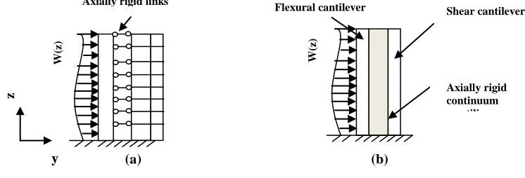
A planar wall-frame is typically presented in figure 2.a. Since, in a non-twisting structure, parallel walls and frames translate identically, they may be simulated by a planar linked model.
The analytical solution requires the structure to be represented by a uniform continuous model (figure 2.b), with all components deflecting identically. The connecting members may be represented by a horizontally rigid connecting medium that transmits horizontal forces only and that causes the continuous flexural and shear cantilevers to deflect identically.
(a) (b)
Figure 2. Planar wall-frame structure and continuum analogy
Assuming the properties of the wall and frame members do not change over the height, it can be shown
W(
z)
Flexural cantilever Shear cantilever
Axially rigid continuum cantiliver
z
y
W(
z)
Axially rigid links
(a) (b) (c)
Shear shape
Shear shape
Flexural shape Point of contra-flexure Flexural
(Smith and Coull (1991) that the linked shear-flexure beam model (figure 2) has the following characteristic differential equation for the deflections:
y
''''
2y
''
w
(
z
)
EI
(12)where 2GA/EI ,
) / 1 / 1 (
12 C G h
EI GA
,G
Ig L and C
Ic hIn the above equations, Ig, L girder inertia and span; Ic, h column inertia and height; I core moment of
inertia; E the concrete elastic modulus; w(z) linearly distributed wind pressure and y(z) drift at height z respectively. GA the story-height averaged shear rigidity of the frames, as though it were a shear member with an effective shear area A and a shear modulus G.
The solution of Eq. (12) for linearly distributed external loading w (z) can then be written as:
H z z
H z
z H
z H
z H
H H
H
H EI
H H z w y
6
1 2 sinh
cosh 1 cosh 1 sinh 2
sinh
1 )
(
2
2
4 4
(13)
Description of example tall building structure
The plan of the structure in figure 3 is of a 35-story, 122.5 m-high wall-frame structure. The horizontal resistance to wind acting on its long side is provided by six rigid frame bents and a central core. Given that the core inertia is 313 m4 and the concrete elastic modulus is 2 x 10⁷ kN/m2, it is required to find the
reliability against a maximum wind loading w(z=H) linearly distributed wind pressure with w(z=H)=1.5 kN/m2. The inertia of frame columns and girders is given in Table 1.
The quantity that defines the performance function is selected to be the top displacement of the building. The stochastic variables are the geometrical parameters, the material properties and the wind pressure as described in Table 1. The performance function is
g
(
I
cor,
I
ic1,...,
w
)
y
y
(
z
H
)
whereyrepresents the allowable maximum displacement of the top displacement of the building and the second term is calculated from equation (13) for z=H. The value of y is increased stepwise and for each step, the reliability by means of the MCM, the 2k and the 2k + 1 variants of the PEM and the second variant of the GSSM, is calculated.Table 1: Data for 35 story tall building example
Stochastic variable Symbol Mean, μ Cov Distribution
Core Inertia Icor 313 m4 0.05 N Frame 1 Interior column Iic1 0.083 m4 0.05 N Exterior column Iec1 0.050 m4 0.05 N Girder Ig1 0.011 m4 0.05 N Frame 2 Interior column Iic2 0.050 m4 0.05 N Exterior column Iec2 0.034 m4 0.05 N Girder Ig2 0.005 m4 0.05 N Concrete elastic modulus E 2 x 10⁷ KN/m2 0.15 LN
Maximum wind pressure w(z=H) 1.5 KN/m² 0.37 LN
RESULTS AND DISCUSSION
In this section, the applicability and usefulness of the aforementioned reliability analysis methods are investigated. As previously mentioned, the study example has a mathematical solution using the continuum approach method, which greatly facilitates the implementation of MCM and allows to compare the results with those of the 2K and 2K + 1 PEM variants.
Based on Equation (13) and the traditional MCM, the probability of failure and the reliability index β are found to be Pf =4.05.10-2 and β=1.735, respectively.
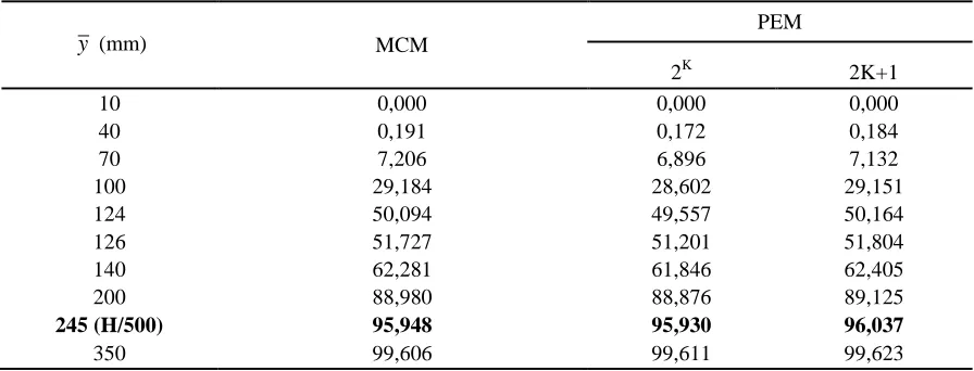
Computing again Pf and β using two PEM variants, very close values are obtained as reported in Table 2.
Table 2: Results of reliability analysis using MCM and the two PEM variants
y (mm) MCM
PEM
2K 2K+1
10 0,000 0,000 0,000
40 0,191 0,172 0,184
70 7,206 6,896 7,132
100 29,184 28,602 29,151
124 50,094 49,557 50,164
126 51,727 51,201 51,804
140 62,281 61,846 62,405
200 88,980 88,876 89,125
245 (H/500) 95,948 95,930 96,037
350 99,606 99,611 99,623
The histogram along with the fitted lognormal PDF using the Monte Carlo simulation technique and the reliability i.e. the CDF of the performance variable calculated using both the MCM and the 2K+1 PEM are displayed in Figures 4 and 5 respectively. MCM results were obtained after performing one hundred thousand evaluations. However, when using the 2k and 2K+1 PEM variants, PEMs results were obtained after only 29=512 evaluations and 2x9+1=19 evaluations, respectively. It is clearly noted that the results are practically coincident.
Figure 4. Histograms for y generated with MCM Figure 5. Reliability for tall building structure examplecalculated by MCM and 2K+1 PEM.
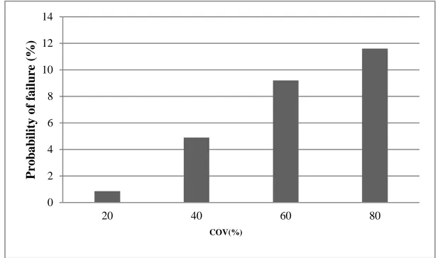
Figure 6. Probability of failure of building structure for different COV of wind loading
Application of GSMM to the tall building example
Thanks to its analytical simplicity, the study example allows to compare the numerical results obtained by MCM and PEMs with those of GSMM.
In this method, a first-order and second-order Taylor series expansion of the performance function around the means of the design variables and parameters is performed (e.g. Harr (1997)), then the definitions of mean and standard deviation are applied, considering all the variables as statistically uncorrelated and the corresponding analytical expression are drawn.
The application of GSMM produces the mean and standard deviation of the output variable, which in this case is the lateral top displacement y(z=H). These statistics are the same as those regarding the performance function g, because they are calculated by differentiating g, and y is a constant value. The values of the statistics are:
0 100 200 300 400 500 600 700 800
0 0.5 1 1.5 2 2.5 3 3.5 4 4.5x 10
4
y(mm)
F
re
q
u
e
n
cy
MC Histogram Lognormal at MC
0 10 20 30 40 50 60 70 80 90 100
0 50 100 150 200 250 300 350 400
R
(%
)
y(mm)
MCM
PEM
0 2 4 6 8 10 12 14
20 40 60 80
Pro
b
a
b
il
ity
o
f
fa
il
u
re
(%
)
GSMM ( first order variant ): mm
y
y 130.5
,
n i x iy x i
y 1 2 mm I y I y I y I y I y I y I y E y w y g ec ic g ec ic cor I g I ec I ic I g I ec I ic I cor E w 52,3 2 2 2 2 2 2 2 2 2 2 2 1 2 2 1 2 2 1 2 2 2 2 2 2 2 2 2 1 1 1
GSMM ( second order variant ):
In case that certain variables have an arbitrary distribution other than the normal distribution, a procedure known as the Rosenblatt transformation is proposed to simplify GSMM second order variant. In this study, we combine GSMM second order variant (Harr (1997)) with the Rosenblatt transformation (Rosenblatt (1952)):
2 2 ² 2 2 ² 2 2 ² 2 1 ² 2 1 ² 2 1 ² 2 ² 2 ² 2 ² 2 1 1 2 ² ! 2 1 2 2 2 1 1 1 ² ² ² ² ² ² ² ² ² ² g ec ic g ec ic co r i I g I ec I ic I g I ec I ic I cor E w n i x i y I y I y I y I y I y I y I y E y w y y x y y mm y 133.6 , mm x x y x y y n i n i n j x x j i x iy i i j
54.1
1 1 1
2 2 2 ! 2 1
The ‘‘deterministic’’ displacement of the top of the building, calculated by setting the nine variables to the corresponding mean values, is y140mm
As one can see, this value does not correspond to the true mean value of the top displacement μy, due to
additional terms containing the standard deviations of some input data. Numerical results of GSMM are given in Table 3. For all the points (y143,3mm
,
y58.3mm).
As a result, the 9-variable problem is reduced to a 4-variable problem. The four variables are: the wind pressure (w), the elastic modulus (E), the core moment of inertia (Icor) and the girder inertia of the interior
frame 1 (Ig1). The four corresponding sensitivity factors are found to be equal to: 0.924, -0.374,-0.058 and
-0,051, respectively.
Table 3: Reliability results of the application of the GSMM to the tall buildingexample
y (mm)
μz βHL R (%)
10 -2,516 -6,450 0,000
40 -1,130 -2,896 0,189
70 -0,570 -1,462 7,190
100 -0,214 -0,547 29,206
124 0,002 0,004 50,163
126 0,018 0,045 51,799
140 0,123 0,315 62,370
200 0,480 1,230 89,058
245 (H/500) 0,683 1,750 95,993
350 1,039 2,664 99,614
For all the points y 54.1mm
Convergence and timing considerations
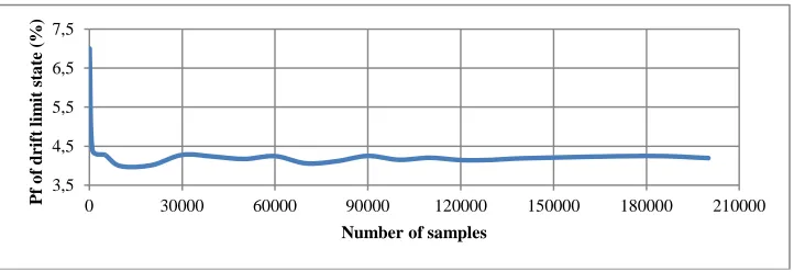
Figure 7. Convergence of probability of failure with increasing sample size
A stochastic analysis with a MC simulation of N runs can be computationally expensive especially for systems with large number of DOF. In the example presented here, this number was fixed at 105 as per the progressive results obtained for the probability of failure as a function of the number of samples. Typical convergence of this response estimate with increasing sample size is illustrated in figure 7. In other cases, however, the slow convergence of statistical processes may require even more iterations. The
savings in computer time achieved with the PEM algorithm become quite evident. In the present study (with nine random input variables and a single random output function chosen as the
performance variable), the first order variant of GSMM was found to be very efficient. The 2k+1 PEM variant required approximately the computational equivalent of only nineteen analysis runs (i.e. 0.09 second for PEM against 16.13 second for the traditional MCM).
CONCLUSIONS
The design process of tall building structures can be significantly impacted by various sources of uncertainties. Nevertheless, it can be performed so as to raise this reliability up to a limit level compatible
3,5 4,5 5,5 6,5 7,5
0 30000 60000 90000 120000 150000 180000 210000
Pf
o
f
d
ri
ft
l
im
it
st
a
te
(
%
)
with structural design code requirements. It is demonstrated that structural reliability is affected by the variability of all uncertain parameters and more importantly by loading randomness and concrete elastic modulus uncertainty. Furthermore, the effects on structural reliability have been shown to be more pronounced for higher variability of the stochastic variables.
In addition, a comparison between the performances of a number of approximate reliability analysis methods was performed. MCM turns out to be the simplest one to implement, with the accuracy of the results depending essentially on the number of samples considered by the designer. Numerical results show, among others, that PEMs and MCM results are found to be in excellent agreement, with MCM requiring significantly greater computational effort for a comparable degree of accuracy. Most interesting of all, is the 2K+1 PEM variant, which was demonstrated to have the fastest performance. Also of particular interest is the first order variant of the GSMM which is found herein to be very efficient and which provides sensitivity information on the stochastic variability of the input variables hence its utility when using a Robust design approach.
As with the GSMM, FORM and SORM methods, the PEM has the important advantage of not requiring the prior knowledge of the probability density functions of input random variables. Contrarily to these methods, PEM has also the distinct advantage of not requiring the need of a differential performance function. Thus, the method can also suitable for the probabilistic analysis of a wide variety of engineering problems.
REFERENCES
Kalos, M.H. and Whitlock, P.A. (2008). Monte Carlo Methods., 2nd ed., New York: Wiley
Hasofer, A.M. and Lind, N.C. (1974). “An Exact and Invariant First Order Reliability Format,” Journal of Engineering Mechanics. Div., ASCE. 100(EMl), 111-121.
Breitung, K. and Hohenbichler, M. (1989). “Asymptotic approximations for multivariate integrals with an application to multinormal probabilities,” J Multivar Anal ,30 80–97.
Christian, J. T. Baecher, G. B. (2002). “The point-estimate method with large numbers of variables,” Int. J. Numer. Anal. Meth. Geomech, 26 1515–1529.
Sorn, P., Gorski, j. and Przewłocki, J., (2015). “Probabilistic Analysis of a Space Truss by Means of a Multidimensional Variable Description,” Archives of Civil Engineering, Poland. 11 99-121. Harr, ME., (1997). Reliability Based Design in Civil Engineering, Dover Publications.
Tiliouine, B. and Chemali B., (2016). “Uncertainty propagation in dynamics of structures with correlated damping using a nonlinear statistical model,” International Journal of Structural Engineering. 7 145 - 159
International Code Council, ( 2009) “International Building Code,”. Whittier, California, USA.
Khuri, A. and Cornell, C.A., (2014). Response Surfaces: design and analyses. 2nd ed. Taylor and Francis.
Farag, R. and Aldar, A. (2016). “A Novel Concept for Reliability Evaluation Using Multiple Deterministic Analysis,” Indian National Academy of Engineering, 1 85–97.
Nowak, S. and Collins, K. R. (2012). Reliability of Structures. 2nd ed. McGraw-Hill Higher Education. Rosenblueth, E. (1981). “Two-point estimates in probabilities,” Appl Math Model, 5 329–335. Smith, B, S. and Coull A. (1991). Tall Building Structures: Analysis and Design. Wiley.
Wilson, E. L. and Habibullah, A., ETABS – Three dimensional analysis of Building Systems, Computers & Structures Inc, Berkeley, USA, 1995.
Rosenblatt, M. (1952) “Remarks on a multivariate transformation,” Ann Math Stat, 23 470–472 Choi, S.K., Grandhi, R, V. and Canfield, R. (2007). Reliability-based Structural Design.