R E S E A R C H
Open Access
High-order conservative Crank-Nicolson
scheme for regularized long wave equation
Kelong Zheng
1and Jinsong Hu
2**Correspondence:
[email protected] 2School of Mathematics and
Computer Engineering, Xihua University, Chengdu, Sichuan 610039, P.R. China
Full list of author information is available at the end of the article
Abstract
Numerical solution for the regularized long wave equation is studied by a new conservative Crank-Nicolson finite difference scheme. By the Richardson
extrapolation technique, the scheme has the accuracy ofO(
τ
2+h4) without refined mesh. Conservations of discrete mass and discrete energy are discussed, and existence of the numerical solution is proved by the Browder fixed point theorem. Convergence, unconditional stability as well as uniqueness of the solution are also derived using energy method. Numerical examples are carried out to verify the correction of the theory analysis.MSC: 65M06; 65N30
Keywords: RLW equation; conservative difference scheme; Richardson
extrapolation; stability; convergence
1 Introduction
Consider the initial boundary value problem for the regularized long wave (RLW) equation
ut+ux+uux–uxxt= , x∈(xL,xR),t∈(,T] (.)
with an initial condition
u(x, ) =u(x), x∈[xL,xR], (.)
and a boundary condition
u(xL,t) =u(xR,t) = , t∈[,T], (.)
whereu(x) is a given known function. The RLW equation is originally introduced as an
alternative to the Korteweg-de Vries (KdV) equation to describe the behavior of the undu-lar bore by Peregrine [] and plays a very important role in physics media, since it describes phenomena with weak nonlinearity and dispersion waves, including nonlinear transverse waves in shallow water, ion-acoustic and magneto hydrodynamic waves in plasma and phonon packets in nonlinear crystals. When it is used to model waves generated in a shal-low water channel, the variables are normalized in the folshal-lowing way: distancexand water elevationuare scaled to the water depthh, and timetis scaled to
h
g, wheregis the
celeration due to gravity. The physical boundary requires
u→, as|x| → ∞. (.)
So, if –xL andxR, problems (.)-(.) is in accordance with the Cauchy problem of equation (.). The RLW equation has the following conserved laws,
Q(t) =
xR
xL
u(x,t)dx=
xR
xL
u(x)dx=Q() (.)
and
E(t) =uL+uxL =uL+(u)x
L=E(), (.)
whereQ() andE() are two positive constants which relate to the initial condition. Existence and uniqueness of the solution of the RLW equation are given in []. Its analytical solution was found [] under restricted initial and boundary conditions, and, therefore, it became interesting from a numerical point of view. Some numeri-cal methods for the solution of the RLW equation such as variational iteration method [, ], finite-difference method [–], Fourier pseudospectral method [], finite element method [–], collocation method [] and adomian decomposition method [] have been introduced in many works. In [], Li and Vu-Quoc pointed out that ‘in some ar-eas, the ability to preserve some invariant properties of the original differential equa-tion is a criterion to judge the success of a numerical simulaequa-tion.’ Meanwhile, Zhanget al.[] thought that the conservative difference schemes perform better than the conservative ones, and the conservative difference schemes may easily show non-linear ‘blow-up.’ Hence, constructing a conservative difference scheme for the numerical solution of the nonlinear partial differential equation is quite significant. In this paper, coupled with the Richardson extrapolation, a two-level nonlinear Crank-Nicolson finite difference scheme for problems (.)-(.), which has the accuracy ofO(τ+h) without
refined mesh is proposed. The scheme simulates two conserved quantities (.) and (.) well, respectively. Moreover,prioriestimate, existence and uniqueness of the numerical solutions are discussed. Convergence and unconditional stability of the scheme are also proved.
The outline of the paper is as follows. In Section , a nonlinear conservative difference scheme is proposed. In Section , we prove the existence of the difference solution by the Browder fixed point theorem.Prioriestimate, convergence and stability are proved in Section , and numerical experiments to verify the theoretical analysis are reported in Section .
2 Nonlinear finite difference scheme
As usual, let h = xR–xL
J be the step size for the spatial grid such that xj =xL +jh (j= –, , , . . . ,J,J+ ). Let τ be the step size for the temporal direction tn=nτ (n= , , , . . . ,N),N= [T
τ]. Denoteu
n
j ≈u(xj,tn) and
Zh=u= (uj)|u–=u=uJ=uJ+= ,j= , , , . . . ,J
Define
In the paper, Cdenotes a general positive constant which may have different values in different occurrences.
The following Crank-Nicolson conservative difference scheme for problems (.)-(.) is considered,
Theorem . Scheme(.)-(.)admits the following invariants,i.e.,
Proof Multiplying (.) withh, then summing up forjfrom toJ– , by boundary condi-tion (.) and formula of summacondi-tion by parts [], we have
and
Substituting (.)-(.) into (.), we have
un+–un+
To prove the existence of solution for scheme (.)-(.), the following Browder fixed point theorem should be introduced. For the proof, see [].
Lemma . Let H be a finite dimensional inner product space.Suppose that g:H→H is continuous,and there exists anα> such thatg(x),x> for all x∈H withx=α. Then there exists x∗∈H such that g(x∗) = andx∗ ≤α.
Theorem . There exists un∈Z
h satisfying difference scheme(.)-(.).
Proof Use the mathematical induction. Obviously, with condition (.), the solution exists forn= . Suppose that forn≤N– ,u,u, . . . ,unsatisfy (.)-(.), then we prove that there existsun+satisfying (.)-(.).
Define an operatorgonZhas follows:
Taking the inner product of (.) withv, we get
vxˆ,v= , v¨x,v= , ϕ(v),v
= , κ(v),v= .
From Lemma . and Cauchy-Schwarz inequality, we get
≥ v–un+
4 Prioriestimate, convergence and unconditional stability
Letv(x,t) be the solution of problems (.)-(.) andvn
j =v(xj,tn), then the truncation error of scheme (.)-(.) is obtained as follows:
rnj =vnjt–
According to Taylor expansion, we obtain the following result.
Theorem . |rn
j|=O(τ+h)holds asτ,h→.
Proof Sincev(x,t) is the solution of problems (.)-(.), we have
vt+vx+vvx–vxxt= , x∈(xL,xR),t∈(,T]. (.)
Firstly, considering the termvt, by Taylor expansion at the point (xj,tn+
), we get
Similarly, by Taylor expansion, we can obtain the following results, respectively:
(vx)| problems(.)-(.)satisfies
uL≤C, uxL≤C, uL∞≤C.
Proof It follows from (.) that
E(t) =uL+uxL=E() =C,
which yields
uL≤C, uxL≤C.
Lemma . Suppose that u∈H[xL,xR],then the solution of scheme(.)-(.)satisfies
un≤C, unx≤C, un∞≤C
for n= , , . . . ,N.
Proof It follows from Theorem . and Lemma . that
un+unx≤En=un+ u
n x
– u
n ˆ x
=C,
that is,
un≤C, unx≤C.
By discrete Sobolev inequality [], we haveun
∞≤C.
Theorem . Suppose that u∈H[xL,xR],then the solution unof difference scheme(.)
-(.)converges to the solution of problems(.)-(.)with order O(τ+h)by the · ∞ norm.
Proof Letting
enj =vnj –unj,
and subtracting (.)-(.) from (.)-(.), respectively, we have
rnj =enjt–
enjx¯xt+
enjˆxˆxt+
en+ j
ˆ x
–
en+ j
¨ x+ϕ
vn+ j
–ϕun+ j
–κvn+ j
+κun+ j
, j= , , . . . ,J– ;n= , , . . . ,N– , (.)
ej = , ≤j≤J, (.)
en∈Zh, n= , , , . . . ,N. (.)
Computing the inner product of (.) with en+, and using boundary condition (.),
we get
rn, en+=en t +
e
n x
t – e
n ˆ x
t + e
n+
ˆ x ,e
n+–
e n+
¨ x ,en+
+ ϕvn+–ϕun+,en+– κvn+–κun+,en+. (.)
Similarly to (.), we have
en+ ˆ x ,e
n+= , en+ ¨ x ,en+
According to Lemma ., Lemma ., Theorem . and Cauchy-Schwartz inequality, we
Substituting (.)-(.) into (.), we get
By discrete Gronwall inequality [], we have
en≤Oτ+h, enx≤Oτ+h.
Finally, by discrete Sobolev inequality [], we get
en∞≤Oτ+h.
This completes the proof of Theorem ..
Similarly, we can prove the stability and uniqueness of the difference solution.
Theorem . Under the conditions of Theorem.,the solution of scheme(.)-(.)is stable by the · ∞norm.
Theorem . The solution unof scheme(.)-(.)is unique.
5 Numerical experiments
In this section, we compute a numerical example to demonstrate the effectiveness of our difference scheme. The single solitary-wave solution of RLW equation (.) is given by
u(x,t) =Asech(kx–ωt+δ), (.)
where
A= a
–a, k=
a
, ω= a ( –a),
anda,δare constants.
Scheme (.)-(.) is a nonlinear system of equations which can be solved by the Newton iteration. Takea=,δ= , and the initial function of problems (.)-(.) is rewritten as
u(x, ) =sech
x
.
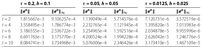
In the numerical experiments, we takexL= –,xR= andT= . The errors in the sense ofL∞-norm andL-norm of the numerical solutions under different mesh steps
handτ are listed in Table . Table shows that the computational and the theoretical orders of the scheme are very close to each other. Furthermore, since we have shown in
Table 1 The errors estimates of numerical solution with varioushandτ
τ= 0.2,h= 0.1 τ= 0.05,h= 0.05 τ= 0.0125,h= 0.025
en en
∞ en en∞ en en∞
t= 2 1.815667e–3 9.106257e–4 1.139049e–4 5.714576e–6 7.120731e–6 3.572519e–6
t= 4 3.558495e–3 1.786774e–3 2.232765e–4 1.121945e–4 1.395820e–5 7.013983e–6
t= 6 5.186555e–3 2.536722e–3 3.254965e–4 1.592516e–4 2.034878e–5 9.955996e–6
t= 8 6.691763e–3 3.175770e–3 4.200524e–4 1.994228e–4 2.626042e–5 1.246776e–5
Table 2 The numerical verification of theoretical accuracyO(τ2+h4)
en(h,τ)/e4n(h 2,
τ
4) e
n(h,τ)
∞/e4n(h2, τ 4)∞ τ= 0.2,
h= 0.1
τ= 0.05,
h= 0.05
τ= 0.0125,
h= 0.025
τ= 0.2,
h= 0.1
τ= 0.05,
h= 0.05
τ= 0.0125,
h= 0.025
t= 2 - 15.940202 15.996241 - 15.935139 15.995926
t= 4 - 15.937612 15.996078 - 15.925675 15.995839
t= 6 - 15.934289 15.995869 - 15.929016 15.995554
t= 8 - 15.930779 15.995648 - 15.924811 15.995067
t= 10 - 15.927366 15.995430 - 15.917690 15.993525
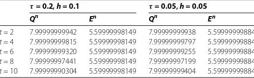
Table 3 Discrete mass and discrete energy with varioushandτ
τ= 0.2,h= 0.1 τ= 0.05,h= 0.05
Qn En Qn En
t= 2 7.99999999942 5.59999998149 7.99999999938 5.59999999884
t= 4 7.99999999815 5.59999998149 7.99999999797 5.59999999884
t= 6 7.99999999320 5.59999998149 7.99999999255 5.59999999884
t= 8 7.99999997441 5.59999998149 7.99999997199 5.59999999884
t= 10 7.99999990304 5.59999998149 7.99999999404 5.59999999884
Theorem . that the numerical solutionunsatisfies invariants (.) and (.), respectively, Table is also presented to show the conservative laws of discrete massQnand discrete energyEn.
From these computational results, the stability and convergence of the scheme are ver-ified, and it shows that our proposed algorithm is effective.
Competing interests
The authors declare that they have no competing interests.
Authors’ contributions
The paper is a joint work of all authors who contributed equally to the final version of the paper. All authors read and approved the final manuscript.
Author details
1School of Science, Southwest University of Science and Technology, Mianyang, Sichuan 621010, P.R. China.2School of
Mathematics and Computer Engineering, Xihua University, Chengdu, Sichuan 610039, P.R. China.
Acknowledgements
The authors would like to thank the editor and the anonymous reviewers for their constructive comments and suggestions to improve the quality of the paper. This work is supported by the Scientific Research Fund of Sichuan Provincial Education Department (No. 11ZB009) and the Doctoral Program Research Fund of Southwest University of Science and Technology (No. 11zx7129).
Received: 21 July 2013 Accepted: 11 September 2013 Published:07 Nov 2013 References
1. Peregrine, DH: Long waves on beach. J. Fluid Mech.27, 815-827 (1967)
2. Bona, JL, Bryant, PJ: A mathematical model for long waves generated by wave makers in nonlinear dispersive systems. Proc. Camb. Philos. Soc.73, 391-405 (1973)
3. Wazwaz, AM: Analytic study on nonlinear variants of the RLW and the PHI-four equations. Commun. Nonlinear Sci. Numer. Simul.12, 314-327 (2007)
4. Soliman, AA: Numerical simulation of the generalized regularized long wave equation by He’s variational iteration method. Math. Comput. Simul.70, 119-124 (2005)
5. Yusufoglu, E, Bekir, A: Application of the variational iteration method to the regularized long wave equation. Comput. Math. Appl.54, 1154-1161 (2007)
6. Chang, Q, Wang, G, Guo, B: Conservative scheme for a model of nonlinear dispersive waves and its solitary waves induced by boundary motion. J. Comput. Phys.93, 360-375 (1991)
7. Ramos, JI: Explicit finite difference methods for the EW and RLW equations. Appl. Math. Comput.179, 622-638 (2006) 8. Zhang, L, Chang, Q: A new finite difference method for regularized long wave equation. J. Numer. Methods Comput.
Appl.21, 247-254 (2000)
10. Alexender, ME, Morris, JL: Galerkin method applied to some model equations for nonlinear dispersive waves. J. Comput. Phys.30, 428-451 (1979)
11. Esen, A, Kutluay, S: Application of a lumped Galerkin method to the regularized long wave equation. Appl. Math. Comput.174, 833-845 (2006)
12. Gu, H, Chen, N: Least-squares mixed finite element methods for the RLW equations. Numer. Methods Partial Differ. Equ.24, 749-758 (2008)
13. Mei, L, Chen, Y: Numerical solutions of RLW equation using Galerkin method with extrapolation techniques. Comput. Phys. Commun.183, 1609-1616 (2012)
14. Soliman, AA, Hussien, MH: Collocation solution for RLW equation with septic spline. Appl. Math. Comput.161, 623-636 (2005)
15. El-Danaf, TS, Ramadan, MA, Abd Alaal, FEI: The use of adomian decomposition method for solving the regularized long-wave equation. Chaos Solitons Fractals26, 747-757 (2005)
16. Li, S, Vu-Quoc, L: Finite difference calculus invariant structure of a class of algorithms for the nonlinear Klein-Gordon equation. SIAM J. Numer. Anal.32, 1839-1875 (1995)
17. Zhang, F, Victor, MP, Luis, V: Numerical simulation of nonlinear Schrödinger systems: a new conservative scheme. Appl. Math. Comput.71, 165-177 (1995)
18. Zhou, Y: Application of Discrete Functional Analysis to the Finite Difference Method. Inter. Acad. Publishers, Beijing (1990)
19. Browder, FE: Existence and uniqueness theorems for solutions of nonlinear boundary value problems. Proc. Symp. Appl. Math.17, 24-49 (1965)
10.1186/1687-1847-2013-287