Volume 2010, Article ID 315381,9pages doi:10.1155/2010/315381
Research Article
Simulations of the Impact of Controlled Mobility for
Routing Protocols
Valeria Loscr´ı, Enrico Natalizio, and Carmelo Costanzo
DEIS, University of Calabria, Rende, Via Pietro Bucci, Cubo 42/D, 87036 Arcavacata di Rende (CS), Italy
Correspondence should be addressed to Valeria Loscr´ı,[email protected]
Received 15 June 2009; Accepted 9 November 2009
Academic Editor: Nikos Passas
Copyright © 2010 Valeria Loscr´ı et al. This is an open access article distributed under the Creative Commons Attribution License, which permits unrestricted use, distribution, and reproduction in any medium, provided the original work is properly cited.
This paper addresses mobility control routing in wireless networks. Given a data flow request between a source-destination pair, the problem is to move nodes towards the best placement, such that the performance of the network is improved. Our purpose is to find the best nodes selection depending on the minimization of the maximum distance that nodes have to travel to reach their final position. We propose a routing protocol, the Routing Protocol based on Controlled Mobility (RPCM), where the chosen nodes’ path minimizes the total travelled distance to reach desirable position. Specifically, controlled mobility is intended as a new design dimension network allowing to drive nodes to specific best position in order to achieve some common objectives. The main aim of this paper is to show by simulation the effectiveness of controlled mobility when it is used as a new design dimension in wireless networks. Extensive simulations are conducted to evaluate the proposed routing algorithm. Results show how our protocol outperforms a well-known routing protocol, the Ad hoc On Demand Distance Vector routing (AODV), in terms of throughput, average end-to-end data packet delay and energy spent to send a packet unit.
1. Introduction
There are many challenges to face while designing wireless networks and protocols, such as obtaining a good through-put, minimizing data delay, and minimizing energy waste. In fact, most of the wireless networks are characterized by battery-equipped devices; thus the minimization of the energy consumption is a key factor. With the miniaturization of computing elements, we have seen many mobile devices appear in the market that can collaborate in an ad hoc fashion without requiring any previous infrastructure con-trol. This gave birth to the concept of self-organization for wireless networks, which is intrinsecally tied to the capability of the nodes to move to different placements. In the last few years, the research community has become interested in the sinergic effect of mobility and wireless networks. Controlled mobility is a new concept for telecommunication research field and can be defined as a kind of mobility where mobile devices are introduced in the network and move to specified destinations with defined mobility patterns for specific objectives. In practice, controlled mobility is a new
the path discovery phase incurs in high energy costs. On the other hand, our system is quasi-static, in the sense that the only mobility we consider is controlled mobility, which is used by nodes to reach specific locations; then, for energy efficiency matters, it is convenient to use a table-driven system. Another interesting routing protocol is [5], where the minimum metric paths are based on two different power metrics:
(i) minimum energy per packet, (ii) minimum cost per packet.
However, this routing algorithm does not take into account the mobility as a new design dimension. In this paper, we take the controlled mobility into account by investigating the performance of a wireless network, where all the devices are equipped with mobility unit. The idea is to use existing multihop routing protocol; specifically we consider the well-known routing algorithm AODV and achieve further improvements in terms of network performance as throughput, data delay, and energy spent per packet, by explicitly exploiting mobility capabilities of the wireless devices. Previous analytical results formulated in [6–8] suggests that controlled mobility of nodes helps to improve network performance. Based on these results, we consider jointly controlled mobility and routing strategies. We perform simulations through a well-known simulation tool [9] to quantify the throughput, delay, and energy spent per packet compared with wireless network where AODV is used. The rest of the paper is organized as follows.Section 2 is the related works. We give some practical application example inSection 3. We give details about Routing Protocol based on Controlled Mobility in Section 4. Section 5 is related to simulation, and finally we conclude our work in Section 6.
2. Related Work
In the recent past a lot of works studied the effects of mobility in the networks. Often, devices’ mobility has been regarded as a negative fact that causes link break, disconnections, and so forth. From a certain moment it has been understood that mobility of nodes can potentially be used to improve perfomance of the network. Grossglauser and Tse [10] showed that mobility increases capacity of a network. Unfortunately, they did not take into account the delay in their work. The research community investigated throughly the delay-throughput trade-offand some interesting results have been obtained. In fact, Gamal et al. [11] determined the throughput-delay trade-off in a fixed and mobile ad hoc network. He showed that, for n nodes, the following statement holdsD(n) = Ω(nT(n)), where D(n) andT(n) are the delay and the throughput, respectively. For a network consisting of mobile nodes, he showed that the delay scales as Ω(n1/2/v(n)), where v(n) is the velocity of the mobile nodes. Once the trade-off between delay and throughput has been characterized, some algorithms that attain the optimal delay for each throughput value have been proposed. Another model makes it possible to exploit the random
3. Practical Applications of Controlled Mobility
In this section we will give some practical applications of Controlled Mobility. There is an interesting real application of controlled mobility to reduce power consumption realized by Intel, that showed that a few motes equipped with 802.11 wireless capabilities can be added to a sensor network in order to act as wireless hubs [19]. Load balancing through controlled mobility in wireless sensor networks is studied by Luo and Hubaux in [1]. The nodes closest to the base station are the bottleneck in the forwarding of data. A base station, which moves according to an arbitrary trajectory, continuously changes the closest nodes and solves the problem. The authors find the best mobility pattern for the base station in order to ensure an even balance of network load on the nodes. Recently, Intel installed a small sensor network in a vineyard in Oregon and a second one in Northern California to monitor microclimates and Redwood canopies, respectively. In this context, the mobile sensors had to measure, share, and combine the collected data regarding temperature, humidity, and other factors. At the gateway, the data was interpreted and used to help avoid mold, frostbite, and other agricultural problems. The agricultural environment is just an example of how a sensor network can take advantage of mobile robot’s capabilities for data gathering and interpretation. Furthermore, sensors often need to be recalibrated and a robot could act as a gateway to the sensor network and perform calibration tasks. An interesting application of sensor devices with mobile robots, related to coverage, is for people with disabilities [20,21]. In fact, technical devices, such as mobile robots, can aid personal assistance. A mobile robot requires a sensing system in order to control the path of movement and the surrounding environment. The robot can be equipped with sensors for detecting distances and obstacles. Another work worth mentioning has been conducted by Kansal et al. in [22]. The authors do not present an algorithm for the opti-mization of some parameters; instead they propose Morph as a new vision of sensor networking, where controlled mobility is considered as an additional design dimension of the communication protocols. They argue that, in Morph, controlled mobility can be employed for the sustainability of the network, which consists in both alleviating the lack of resources and improving the network performance.
4. A New Routing Protocol Based on
Controlled Mobility (RPCM)
The network scenario we consider consists of all nodes able to move and control their movements. The communication strategy used in this work considers different paths for each pair source-destination nodes and the best path is selected to be used for data communication. The choice of the best path is based on a metric. Specifically, in this context we consider the path whose nodes have to travel the total minimum distance to reach the evenly spaced positions on the straight line between the source-destination pair. The same metric has been proposed in an optimization model in [8], where the model determines the placement that minimizes the
Transport layer
Network layer
Data link layer
Physical layer
C
ross
la
yer
int
eg
ra
tion
for
mobilit
y
management
Figure1: Protocols’ stack integrated with mobility management.
total travelled distance of the sensor nodes. This kind of movement could be useful in all situations where a mobility too high can be dangerous (i.e., military applications such as minefields monitoring) or difficult because of a high presence of obstacles.
4.1. Some Assumptions. Assume that n nodes deployed randomly in a square area. All the nodes have the same transmission range. If two nodes are within each other’s transmission range, they can communicate directly and they areneighbours. Otherwise they have to rely on intermediate nodes to relay the messages for them. Any node in the network may have data to be sent to any other node. The path from a source to a destination may not be direct but involves other intermediate nodes. We assume that several paths, from the sourcesto the destinationd, have already been discovered by a routing protocol. Specifically, we apply the Route Request phase of the AODV protocol, with some additional information such as the nodes’ position. We need this information for implementing our protocol as explained in the follow. We also assume that nodes move only in order to reach specific locations when they belong to a path. Our mobility control scheme is not directly incorporated into a specific layer of the classical ISO/OSI layer structure (i.e., physical layer, routing layer, etc.) but is orthogonal to this kind of subdivision as we can observe in Figure 1. In fact, controlled mobility could be exploited at different levels.
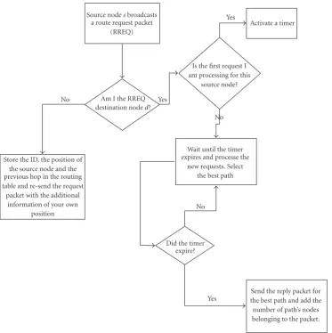
Store the ID, the position of the source node and the previous hop in the routing table and re-send the request
packet with the additional information of your own
position
Source nodesbroadcasts a route request packet
(RREQ)
Is the first request I am processing for this
source node? Am I the RREQ
destination noded?
Wait until the timer expires and processe the
new requests. Select the best path
Send the reply packet for the best path and add the number of path’s nodes belonging to the packet. Yes
Yes No
No
No
Yes Did the timer
expire?
Activate a timer
Figure2: Routing Request phase of RPCM.
processing other requests. In order to avoid unuseful delay, a destination node will wait for a specific time, and then it will send a reply packet by building the best selected path. The metric we introduced to evaluate the goodness of a path is based on the total travelling distance. In practice, the algorithm will choose the path that minimizes the sum of nodes’ travelled distances. Other metrics, such as the minimization of the maximum travelled distance, could be considered and implemented. InFigure 2the request phase of the routing protocol is explained. We can observe that the source node starts a request phase by sending a Route Request and every intermediate node stores the position of the previous node, the ID of the previous node, and rebroadcasts the request packet. The mechanisms to avoid loop and control packet storms are the same as in AODV. Once the Request Packet reaches the destination node, if the request is processed for the first time, the destination node d activates a timer and continues to process other Request Packets of the same source node s. Otherwise, d compares the previous path with the current path and selects the best one (in this case the path whose nodes travel the minimum total distance). Once the timer expires, d sends
a Reply Packet to the first node of the selected path in the backward direction. This node computes its new position depending on the number of nodes involved in the path (this information is sent from thednode) and forwards the Reply Packet to the following node in the backward direction (this information has been stored in the Routing Table during the Route Request phase). Hence, this node will move to the evenly spaced position on the straight line between the source and the destination. When each relay node knows its position, the optimal configuration of relay nodes for an active flow is established as in [6, 23]. It is worth to note that in this case the solutions found in [6,23] are the same, because the initial energy of nodes is the same. In practice, the nodes will reach the evenly spaced positions on the straigth line between the source and the destination. In Figure 3the Reply phase is explained. Once the source nodes receives the Reply Packet, all the nodes belonging to the path have already moved to their new position andswill start the data communication flow.
Send the reply packet with information of
the best path
I am the destination
noded.
Wait until the timer expires. Did the timer
expire?
Am I the source nodes?
You belong to the new path. Compute your new position based on the total number of intermediate
nodes between source and destination. Send bacwardly the
reply packet and move to reach your new location
Source and destination communicate until the end of
data flow Start the data
flow communication
No
No Yes
Yes
Figure3: Reply phase of RPCM.
line between the source and the destination. The Mobility Algorithm can be summarized as follows.
Mobility Algorithm. Mobility control at each relay node. (i) Each node acquires the information of the new
position it has to reach when the reply of the request is received. The new position is on the straight line between the source and the destination and each node will be positioned in an evenly distributed fashion.
(ii) Each node that received a reply packet moves towards its new position.
In [23], authors had to introduce a damping factor g to avoid oscillations in the network. In fact, nodes exchange local position information with neighbours and some iteration of the distributed algorithm is needed to reach the final optimal displacement of the nodes. Thus, we do not
need to introduce any damping factor, because nodes already have all the information they need to reach the new location. Furthermore, we do not have any convergence concern. In fact, nodes start to move once they receive the reply packet and reach the final destination.
From the description of the routing protocol is clear the reason why no damping factor is needed, even if our protocol is totally distributed and the Mobility Control Algorithm is orthogonal to the network layer. The new protocol requires few changes to the classical schemes; the information that need to be added are as follows:
(i) in the Request Packet: the positions and the IDs of source and forwarding nodes;
(ii) in the Reply Packet: the positions of the destination node and the hop number of the source-destination path;
3
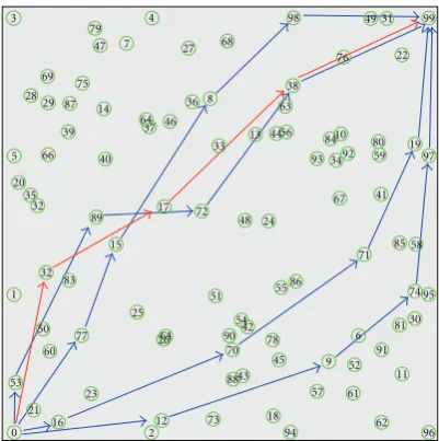
Figure4: A snapshot of the network before applying the Routing Protocol.
Figure5: A snapshot of the network after RPCM is applied.
The effect of applying the RPCM protocol is shown in Figures4and5.
In Figure 4 we can observe the selection of many potential paths for the pair source-destination, nodes 0 and 99, respectively. Specifically, the paths discovered are 0-53-89-72-38-99, 0-77-15-8-98-99, 0-16-70-71-19-99, 0-12-9-74-97-99, and 0-32-17-38-99. Among the different paths, the one whose nodes travel the total minimum distance is chosen. In this case the selected path based on our metric is 0-32-17-38-99. When the reply phase begins, the first node that receives the reply packet is node 38, it computes its new location and sends the reply packet to the node 17, and then it moves towards its best location. In similar fashion, node 17 receives the reply packet from the node 38, computes its new destination, sends the reply packet and moves to the new location, and so forth. Once node 0 receives the reply packet
from the node 32, then all the nodes belonging to the path (in this case, nodes 38, 17, and 32) already moved to their new positions and node 0 starts the data communication flow to node 99. Note that source node and destination do not move.
5. Simulation and Results
As we already said in the previous subsections, the optimiza-tion model including the minimizaoptimiza-tion of the nodes’ total travelled distances along with other possible metrics has been introduced in [8]. Unfortunately in that analytical work, many practical details could not be taken into consideration. For this reason, we chose to implement one of those possible metrics in a complete routing algorithm and simulate its behaviour in a well-known network simulator: ns2, in order to evaluate the realistic effects of controlled mobility in the routing process in comparison with the AODV protocol.
5.1. Reference Environment. InTable 1, all the most impor-tant environment and simulator parameters are reported. We chose to implement our algorithm in a square area of 500 m×500 m, where a variable number of wireless nodes has been randomly deployed, according to the reported nodes density (2, 3, 4, 5, 6 (nodes/m2), which correspond to 50, 75, 100, 125, 150 nodes). Also the number of concurrent flows is considered variable. Depending on the density, nodes have a different transmission area to cover. All nodes have initially the same energy and transmit at the same trans-mission rate; when they move, the energy expenditureEMis proportional to the travelled distancedby a movement factor k. When nodes mobility is allowed, the set of limitations becomes enriched with new elements. In fact, the definitions of an energy model related with the motion of nodes and of another model related with the communication needed for their coordination are required. For the former a simplified model is a distance proportional modelEM(d) = kd+γ, wheredis the distance to cover,k[J/m] takes into account the kinetic friction; whileγ[J] represents the energy necessary to win the static friction, both these constants depend on the environment (harsh or smooth ground, air, surface or deep water). For the latter, usually the energy required to send one bit at the distance d is EC(d) = βdα, whereα is the exponent of the path loss (2 ≤ α ≤ 4) depending on the environment andβis a constant [J/(bitsmα)]. Regarding the simulator, we used a two-ray ground propagation model and both the simulated routing protocols (AODV and RPCM) are mounted on top of the IEEE 802.11 MAC. The energy spent in sleep, wake-up, and active mode is reported in the table. The output parameters taken in consideration are as follows:
(i) throughput,
(ii) delay,
(iii) energy spent for received packet.
60 65 70 75 80 85 90 95 100
Thr
o
ug
hput
(%)
2 3 4 5 6
Nodes density (nodes/m2) ×10−4
AODV RPCM
Figure6: Performance of AODV and RPCM in terms of through-put, whenf =6.
0 0.5 1 1.5
Dela
y
(s)
2 3 4 5 6
Nodes density (nodes/m2) ×10−4
AODV RPCM
Figure 7: Performance of AODV and RPCM in terms of delay, when f=6.
5.2. Performance Evaluation. We performed two simulation campaigns: the first consists of increasing nodes density for a fixed number of flows (f =6), in the second the number of flows varies between 4 and 12 and the nodes density is set to ρ=4 (nodes/m2). Figures6,7, and8show the performance of the two algorithms for the first simulation campaign in terms of throughput, delay and energy spent for received packed, respectively.
As we can see, for all the output parameters our scheme out performs the AODV achieving 30%, 80% and 40% of improvements for throughput, delay and energy spent for received packet, respectively. Furthermore, the behavior of the RPCM scheme is more robust and scalable than the
0.006 0.007 0.008 0.009 0.01 0.011 0.012 0.013 0.014
Energ
y
spent
for
rec
ei
ve
d
p
ac
ke
t
(J)
2 3 4 5 6
Nodes density (nodes/m2) ×10−4
AODV RPCM
Figure8: Performance of AODV and RPCM in terms of energy spent for received packet, whenf =6.
30 40 50 60 70 80 90 100
Thr
o
ug
hput
(%)
4 6 8 10 12
Flows numbers AODV
RPCM
Figure9: Performance of AODV and RPCM in terms of through-put, whenρ=4 (nodes/m2).
AODV, since it is almost constant for all output parameters when density, while in the AODV scheme, delay and energy spent are affected by the nodes density.
Figures 9,10, and11show the performance of the two algorithms for the second simulation campaign in terms of throughput, delay and energy spent for received packed, respectively.
0 0.5 1 1.5 2 2.5 3 3.5 4 4.5
Dela
y
(s)
4 6 8 10 12
Flows numbers AODV
RPCM
Figure10: Performance of AODV and RPCM in terms of delay, whenρ=4 (nodes/m2).
0.005 0.01 0.015 0.02 0.025 0.03
Energ
y
sp
ent
for
re
ce
iv
ed
pa
ck
et
(J
)
4 6 8 10 12
Flows numbers AODV
RPCM
Figure11: Performance of AODV and RPCM in terms of energy spent for received packet, whenρ=4 (nodes/m2).
the number of concurrent flows, until it is below 6, the performance is constant with very high throughputs and very low delays, when the number of flows is higher than 6, then the performance worsens.This result gives the designer a good hint about the number of concurrent flows to allow into the network, in order to have high performance. At least, the energy spent for received packet shows two different trends for AODV and RPCM, the first is not very affected by the number of flows and oscillates between 0.012 and 0.015 J, while the second shows a negative exponential bahavior for f =4 the energy spent on average is 0.025 J but it reduces till 0.005 J when the number of flows increases.
Table1: Evaluation parameters.
Environment
Field Area (L×L) 500 m×500 m
Nodes Density (ρ) [2÷6]·10−4(nodes/m2)
Flows Number (f) [4÷12]
Maximum Transmission Radius (r) 1/(2√ρ) m Initial Residual Energy Range (Ei) 100 J
Transmission Rate (rT) 32 kb/s
Movement Constant (k) 0.1 J/m
Simulator
Propagation Model Two-Ray Ground
MAC Type IEEE 802.11
Packet Size 512 byte
set val(rxPower) 0.00175 W
set val(txPower) 0.00175 W
Wake-Up Time 0.005 s
Number of runs 10
Statistical confidence interval 95%
6. Conclusion
In this work we focused on both the novel concept of controlled mobility and the routing algorithms. The concept of controlled mobility has been introduced in some previous recent work, but it has only been considered from an analytical point of view or in a marginal fashion, such as only a mobile base station in the network. In this paper we focus on the controlled mobility as a new design dimension and we exploit it by implementing a new routing protocol based on controlled mobility. The most important aspect of this is related to the evaluation performance based on the usage of a well-known simulation tool, ns2. In fact, in previous works the analytical approach limited the use of controlled mobility while in this context, thanks to the simulator, we have been able to consider many realistic aspects of the network, while a routing protocol is implemented. Extensive simulations have been conducted and simulation results have shown how the new routing protocol outperforms a well-known routing algorithm, the AODV. Furthermore, results obtained suggest that other metrics can be easily realized and tested by simulation. In fact, as future works, we intend to study other optimization metrics such as the maximization of the network lifetime or the minimization of the average (or the maximum) distance travelled by nodes belonging to a path.
References
[1] J. Luo and J.-P. Hubaux, “Joint mobility and routing for lifetime elongation in wireless sensor networks,” inProceedings of the 24th Annual Joint Conference of the IEEE Computer and Communications Societes (INFOCOM ’05), vol. 3, pp. 1735– 1746, Miami, Fla, USA, March 2005.
in Conjunction with the 24th International Conference on Distributed Computing Systems (ICDCS ’04), vol. 24, pp. 698– 703, Tokyo, Japan, March 2004.
[3] C. E. Perkins, E. M. Belding-Royer, and I. Chakeres, “Ad hoc on-demand distance vector (AODV) routing,” inIETF Internet draft, draft-perkins-manet-aodvbis-00.txt, October 2003. [4] V. D. Park and M. S. Corson, “A highly adaptive distributed
routing algorithm for mobile wireless networks,” in Proceed-ings of the 16th Annual Joint Conference of the IEEE Computer and Communications Societes (INFOCOM ’97), vol. 3, pp. 1405–1413, Kobe, Japan, April 1997.
[5] S. Singh, M. Woo, and C. S. Raghavendra, “Power-aware routing in mobile ad hoc networks,” in Proceedings of the 4th Annual IEEE/ACM International Conference on Mobile Compuetr and Network (MOBICOM ’98), pp. 181–190, Dallas, Tex, USA, October 1998.
[6] E. Natalizio, V. Loscr´ı, and E. Viterbo, “Optimal placement of wireless nodes for maximizing path lifetime,”IEEE Communi-cations Letters, vol. 12, no. 5, pp. 362–364, 2008.
[7] E. Natalizio, V. Loscr´ı, F. Guerriero, and A. Violi, “Energy spaced placement for bidirectional data flows in wireless sensor network,”IEEE Communications Letters, vol. 13, no. 1, pp. 22–24, 2009.
[8] V. Loscr´ı, E. Natalizio, C. Costanzo, F. Guerriero, and A. Violi, “Optimization models for determining performance benchmarks in wireless sensor networks,” inProceedings of the 3rd International Conference on Sensor Technologies and Applications (SENSORCOMM ’09), pp. 333–338, Athens, Greece, June 2009.
[9] http://www.isi.edu/nsnam/ns/.
[10] M. Grossglauser and D. N. C. Tse, “Mobility increases the capacity of ad hoc wireless networks,”IEEE/ACM Transactions on Networking, vol. 10, no. 4, pp. 477–486, 2002.
[11] A. El Gamal, J. Mammen, B. Prabhakar, and D. Shah, “Throughput-delay trade-offin wireless networks,” in Pro-ceedings of the 23th Annual Joint Conference of the IEEE Computer and Communications Societes (INFOCOM ’04), vol. 1, pp. 464–475, Hong Kong, March 2004.
[12] N. Bansal and Z. Liu, “Capacity, delay and mobility in wireless ad hoc networks,” in Proceedings of the 22th Annual Joint Conference of the IEEE Computer and Communications Societes (INFOCOM ’03), vol. 2, pp. 1553–1563, San Francisco, Calif, USA, March-April 2003.
[13] R. M. de Moraes, H. R. Sadjadpour, and J. J. Garcia-Luna-Aceves, “Mobility-capacity-delay trade-offin wireless ad hoc networks,”Ad Hoc Networks, vol. 4, no. 5, pp. 607–620, 2006. [14] E. Lee, S. Park, D. Lee, Y. Choi, F. Yu, and S.-H. Kim, “A
pre-dictable mobility-based communication paradigm for wireless sensor networks,” inProceedings of Asia-Pacific Conference on Communications (APCC ’07), pp. 373–376, 2007.
[15] Z. Zhi, D. Guanzhong, L. Lixin, and Z. Yuting, “Relay-based routing protocols for space networks with predictable mobility,” in International Conference on Space Information Technology, vol. 5985 ofProceedings of SPIE, 2005.
[16] S. Merugu, M. Ammar, and E. Zegura, “Routing in space and time in networks with predictable mobility,” Tech. Rep. GIT-CC-04-07, Georgia Institute of Technology, Atlanta, Ga, USA, 2004.
[17] A. Howard, M. Mataric, and G. Sukhatme, “Mobile sensor network deployment using potential field: a distributed scal-able solution to the area coverage problem,” inProceedings of the 6th International Symposium on Distributed Autonomous Robotic Systems (DARS ’02), pp. 299–308, Fukuoka, Japan, June 2002.
[18] D. Wang, J. Liu, and Q. Zhang, “Probabilistic field coverage using a hybrid network of static and mobile sensors,” in
Proceedings of the International Workshop on Quality of Service (IWQoS ’07), pp. 56–64, Chicago, Ill, USA, June 2007. [19] R. M. Kling, “Intel motes: advanced sensor network platforms
and applications,” inProceedings of the IEEE MTT-S Interna-tional Microwave Symposium Digest, vol. 2005, pp. 365–368, Long Beach, Calif, USA, June 2005.
[20] R. M. Mahoney, “Robotic products for rehabilitation: status and strategy,” inProceedings of the International Conference on Rehabilitation Robotics (ICORR ’97), pp. 12–22, The Bath Institute of Medical Engineering, Bath University, Bath, UK, April 1997.
[21] M. J. Topping and J. R. Hegarty, “The potential of low-cost computerised robot arms as aids to independence for people with physical disability,” inProceedings of the 1st International Workshop Domestic Robots and the 2nd International Workshop on Medical and Health Care Robotics, pp. 303–307, London, UK, 1989.
[22] A. Kansal, M. Rahimi, D. Estrin, W. J. Kaiser, G. J. Pottie, and M. B. Srivastava, “Controlled mobility for sustainable wireless sensor networks,” in Proceedings of the 1st Annual IEEE Communications Society Conference on Sensor and Ad Hoc Communications and Networks (SECON ’04), pp. 1–6, Santa Clara, Calif, USA, October 2004.
[23] D. K. Goldenberg, J. Lin, A. S. Morse, B. E. Rosen, and Y. R. Yang, “Towards mobility as a network control primitive,” in