Dynamic rate adaptive MIMO mode switching between spatial multiplexing and diversity

(1)

R E S E A R C H

Open Access

Dynamic rate-adaptive MIMO mode switching

between spatial multiplexing and diversity

Chanhong Kim and Jungwoo Lee

*

Abstract

In this article, we propose a dynamic multiple-input multiple-output (MIMO) mode switching scheme between spatial multiplexing and diversity modes, which also includes adaptive modulation. At each transmission, we select the modulation level and the MIMO mode that maximize the spectral efficiency while satisfying a given target bit error rate. The dynamic MIMO mode scheme considers instantaneous spectral efficiency whereas the conventional static scheme considers only the average SNR. As for adaptive modulation, a new method is proposed to compute the SNR thresholds for adaptive modulation in each MIMO mode, and it can avoid the computational difficulty of the

conventional Lagrangian (optimal) method at high average SNR. To deal with the case where the rates of the two MIMO modes are the same, we also propose a new measure based on the BER exponent, which has lower

computational complexity than a conventional measure. Numerical results show that the proposed dynamic mode switching improves over the conventional static mode switching in terms of average spectral eﬃciency.

Introduction

Today’s wireless communication systems demand high data rate and spectral eﬃciency with increased reliabil-ity. Multiple-input multiple-output (MIMO) systems have been popular techniques to achieve these goals because increased data rate is possible through spatial multiplex-ing scheme [1] or improved diversity order is possible through transmit diversity scheme (e.g., space-time block code, STBC) [2]. Other ways are link adaptation tech-niques, where transmission parameters such as modula-tion and coding are dynamically adapted to the varying channel condition [3]. A typical link adaptation technique is adaptive modulation in which an adequate modulation level is selected by means of the current signal-to-noise ratio (SNR).

Recently, adaptive modulation schemes in conjunction with MIMO techniques have been investigated [4-11]. The prior study in the literature mainly tried to maxi-mize the average spectral eﬃciency (ASE) for only one MIMO mode, either spatial multiplexing [8] or transmit diversity [5-7,11]. In [12], the mode switching between diversity and multiplexing was ﬁrst proposed. But the authors focused on the situation where both MIMO

*Correspondence: [email protected]

School of Electrical Engineering and Computer Science, Seoul National University, Seoul, Korea

modes have equal spectral eﬃciency without considering adaptive modulation, so that they showed the result that spatial multiplexing is preferred in low SNR region. The mode switching scheme combined with adaptive modula-tion was proposed in [9,10], but the analysis was focused on the static mode switching which depends only on the average SNR.

In this article, we propose a dynamic MIMO mode switching scheme which considers instantaneous channel condition in conjunction with rate adaptation. Although the adaptive modulation part is based on the exist-ing methods [5,7-9,11], we compare the performance of the existing techniques, and also propose a sub-optimal method to obtain the SNR thresholds for the average BER constraint. Its complexity is lower than that of the optimal method using a Lagrange multiplier, but the performance degradation is negligible. The proposed mode switching scheme is based on the instantaneous spectral eﬃciency (ISE). In case the ISE’s of the two modes are equal, an additional rule is necessary for mode selection. Although the Demmel condition number proposed in [12] can be a choice, we propose a new method which has lower complexity than the Demmel condition number without performance loss.

This article is organized as follows. In the section of System overview, we outline the system and the chan-nel model as well as the structure of the considered

(2)

MIMO mode switching system. The dynamic MIMO mode switching scheme combined with adaptive mod-ulation is then proposed in the section of rate-adaptive MIMO mode switching. In the section of Simulation results, we compare the performance of the proposed algorithm with that of the existing methods. Since numer-ical methods are necessary in order to get the SNR thresh-olds for the average BER constraint, we shows detailed results in this section. Finally, conclusions are drawn in the last section.

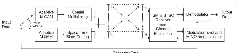
System overview

We consider a MIMO system withMtransmit antennas andN receive antennas. The block diagram of the pro-posed system is shown in Figure 1. The system consists of a transmitter with a switch between a multiplexing and a diversity modulator, a receiver unit with the corre-sponding pair of receivers, a modulation level and mode selector, and a low rate feedback path. At the receiver side, the modulation level and the MIMO mode are selected according to the current channel condition. The informa-tion about the selected modulainforma-tion level and the MIMO mode is sent to the transmitter through the feedback path. The transmitter then switches the MIMO mode with the modulation level based on the feedback information.

Suppose that theN ×Mﬂat fading channel matrixH

has i.i.d. complex Gaussian random entries. The (i,j)th entry [H]i,j= hij is distributed as CN(0, 1)a. The chan-nel is assumed to be quasi-static (chanchan-nel coeﬃcients do not change during one time interval, and change indepen-dently in the next interval). The input-output relation for the MIMO channel is given by

y=

Es

MHs+n, (1)

whereyis theN×1 received signal vector,Esis the average energy per symbol,sis the transmitted signal vector with energyM, i.e.,E[sHs]=Mb, andnis anN×1 i.i.d. com-plex additive white Gaussian noise (AWGN) vector with the distributionCN(0,N0IN). Letρbe the average SNR at the receiver, which is given byρ = Es

N0. We have omitted

the time index in (1) for convenience. We also assume per-fect channel knowledge at the receiver and zero feedback delay.

Rate-adaptive MIMO mode switching

In this article, we propose a new rate-adaptive MIMO mode switching algorithm. The goal is to maximize the ASE while satisfying a given bit error ratio constraint. The proposed algorithm can be summarized by the following three steps.

1. Calculate the post-processing SNR in each MIMO mode.

2. Decide the modulation order in each MIMO mode. 3. Decide one MIMO mode based on a given selection

rule.

For analysis, we consider a linear receiver for the spa-tial multiplexing mode, and orthogonal space-time block codes (OSTBC) for the diversity mode. In Step 2, we ana-lyze several adaptive modulation techniques subject to an instantaneous BER constraint as well as an average one. In Step 3, we propose the mode selection rule based on the ISE as well as the rule which can be applied to the case when both of the two MIMO modes have the same data rate.

Post-processing SNR calculation (Step 1)

The post-processing SNR at the receiver is calculated separately in each MIMO mode with a given detection algorithm. At ﬁrst, in the spatial multiplexing mode, the post-processing SNR of themth (m = 1, 2,. . ., M) out-put data stream of the zero forcing (ZF) receiver, denoted asγm,ZF, is given by ([13], Eq. (7.43))

γm,ZF=

ρ

M

1

HH_H−1 m,m

, (2)

and the SNR of the minimum mean-square error (MMSE) receiver, denoted asγm,MMSE, is given by ([13], Eq. (7.49))

(3)

γm,MMSE=

The post-processing SNR of the OSTBC system, denoted asγOSTBC, is given by

whereζis the code rate of the OSTBC.

Decision of the modulation order (Step 2)

Using the post-processing SNR obtained in Step 1, we can choose an appropriate modulation order for each MIMO mode which enhances spectral eﬃciency without exceeding a given target BER at the receiver. Since adap-tive modulation for one MIMO mode with a given BER constraint has been studied in [4-8,11], we take a simi-lar approach of the literature. For analysis, we consider a discrete rate adaptive system for which the constellations are restricted to a ﬁnite setM= {M0,M1,. . .,ML}with Gray coded quadrature amplitude modulation (QAM), where Ml denotes the constellation size and Ml−1 < Ml, ∀l. The SNR range is subdivided into L+1 bins bounded by the switching thresholdθl(l=0, 1,. . ., L+

1) where θ0 = 0. Let γ be the post-processing SNR.

The receiver chooses the constellationMlwheneverθl≤ γ < θl+1. If γ < θ1, data transmission is suspended for

the corresponding channel since the respective BER con-straint cannot be satisﬁed. Moreover, the maximum SNR threshold is set to inﬁnity, i.e.,θL+1= ∞.

SNR thresholds for instantaneous BER constraint

An easy way to set the switching thresholdsθl’s is to use the instantaneous BER (I-BER). In this approach, the BER of every reception has to be less than or equal to the tar-get BERδ0. In order to meet the constraint, the BER for

a QAM in AWGN channels can be used. Although the exact BER expressions for M-QAM are shown in [14], they are not easily inverted with respect to the SNR, so that a numerical method is necessary. Instead, in the adaptive modulation literature [5-8], an exponential function form is used, which is given by

Pe(γ,Ml)≈alexp(−clγ ), (5)

whereal = 0.2 andclis a constellation speciﬁc constant deﬁned as [4]

If we want a more accurate form than the above approx-imation, we can ﬁnd the modulation speciﬁc constants

al and cl numerically using curve-ﬁtting methods [11]. Table 1 shows those values of M-QAM’s which are used

Table 1 Constellation speciﬁc constants for BER approximation in AWGN channels [11]

Modulation BPSK QPSK 16-QAM 64-QAM

al 0.1978 0.1853 0.1613 0.1351

cl 1.0923 0.5397 0.1110 0.0270

in [11]. Inverting (5) with respect to γ, the switching threshold is determined as

θl= 1

Although it is simple, I-BER approach keeps the instan-taneous BER at all time instants below the target BERδ0.

This is so conservative that the average BER (A-BER) is lower than δ0. In order to make the A-BER be equal to

δ0, SNR thresholds should be lowered. Therefore, there is

potential for improving the ASE by adjusting the switch-ing threshold of each modulation.

SNR thresholds for average BER constraint

Generally, the ASEηfor one channel use is given by

η= L

l=1

bl·pl, (8)

wherebl=log2Mlis the number of bits corresponding to thelth modulation andplis the probability that the post-processing SNR falls into thelth bin, given by

pl=

θl+1

θl

f(γ )dγ, (9)

wheref(γ )is the probability density function (pdf ) of the post-processing SNR. The A-BER can be denoted as the average number of error bitsNe,avg divided by the aver-age number of transmitted bitsNb,avg. It is observed that

Nb,avg=ηby the deﬁnition in (8) andNe,avgis given by

Since it has already been known that the pdf ’s of the two MIMO modes have Gamma distributions, using the above formulas, the ASE and the A-BER can be obtained as closed forms as (26) and (30) in case of ZF spatial multi-plexing system and (34) and (38) in case of OSTBC system, respectively. See Appendix for details. The pdf ofγm,MMSE

(4)

a generalized Gamma distribution [15]. Thus, though it is approximation, the analysis of the MMSE receiver can be done with the same procedure as that of the ZF receiver.

Optimal method In A-BER approach, the goal is to max-imize the ASE under the constraint that the A-BER should be lower than or equal toδ0. Deﬁning the set of adjustable

switching thresholds as = θl |l = 1, 2,. . .,Lc_{, the}

optimization problem can be formulated as

o =arg max

η, subject toPe,avg ≤δ0. (12)

This problem can be solved with a Lagrange multiplier. SincePe,avgis denoted as

convenience, the Lagrangian of (12) is deﬁned as

L(,λ)=η+λ(Ne,avg−δ0η). (14)

Diﬀerentiating (14) with respect toθl and equating to zero, the following relationship for l = 2, 3,. . .,L is

According to the relationship, onceθ1is chosen, all the

otherθl’s are uniquely determined. Thus, the optimal SNR thresholds can be found numerically by adjustingθ1only.

Descending search method (sub-optimal) Intuitively, as the SNR range assigned to a high order modulation increases, the ASE increases while the BER also increases at the same time. Thus, in order to maximize the ASE, the SNR thresholdθlin descending order (l=L,L−1,. . ., 1) has to be lowered as much as possible. Since the A-BER has to be kept belowδ0, we take the constraint thatPe(l)≤

8: Exit for loop. 9: else

In the proposed algorithm, a certain modulation can be completely switched oﬀ because the solution that satisﬁes

Pe(l) =δ0may not exist at all or only higher order

mod-ulations may satisfy the BER constraint on the whole SNR region.

Although the A-BER approach has higher computa-tional complexity than the I-BER approach, the thresholds can be calculated oﬀ-line, and the A-BER approach is still practical.

Dynamic MIMO mode switching (Step 3)

After the modulation order in each MIMO mode is cho-sen, the ISE can be calculated. The ISE of the spatial multiplexing system with ZF receiver, denoted asRZF, can

be written as

where bm,ZF is the number of bits corresponding to the

selected modulation on the mth subchannel. Likewise, the ISE of the OSTBC system, denoted asROSTBC, can be

expressed as

ROSTBC=ζ·bOSTBC (bits/channel use), (17)

wherebOSTBCdenotes the number of bits corresponding to

the selected modulation.

IfRZFandROSTBCare diﬀerent from each other, the mode

selection rule is as follows: ifRZF > ROSTBC, spatial

mul-tiplexing is chosen for the next transmission mode, and vice versa. In case of RZF = ROSTBC, a general rule is to

select a mode that gives lower BER, and the MIMO mode can be chosen based on the following two methods. One method is the Demmel condition number approach which was proposed in [12]. The Demmel condition numberκD is deﬁned as

κD:= HF λmin(H)

, (18)

whereλmin(H)denotes the minimum singular value ofH,

and spatial multiplexing is preferred if

κD≤ dmin,ZF dmin,OSTBC

, (19)

where dmin,ZF is the minimum Euclidean distance of the

transmit constellation of the spatial multiplexing sys-tem with a ZF receiver, and dmin,OSTBC is the minimum

Euclidean distance of the OSTBC system.

Another method is to use the I-BER of each MIMO mode, which can be measured by the exponent of the BER Equation (5). In other words, a MIMO mode which has lower I-BER than the other can be chosen. Assuming that the approximation of the I-BER in (5) and the constella-tion speciﬁc constants in [4] are used, the following rule can be derived. Spatial multiplexing is preferred if

(5)

whereγmin,ZF = min

m γm,ZF, which means that the worst stream of the spatial multiplexing mode is used to calcu-late the I-BER. Although the Demmel condition number can be used for mode switching, it has higher complex-ity than (20) because singular value decomposition is necessary to get κD in (18), whereas (20) only uses the parameters which are already obtained from the previ-ous steps. Therefore, the proposed measure is desirable in terms of computational complexity.

Simulation results

In simulation, a simple MIMO system is considered whose antenna conﬁguration isM= N = 2. Constellations are restricted to M-QAM withM = {1, 2, 4, 16, 64}, where 1 means no transmission, 2 BPSK, 4 QPSK, and so on. The target BERδ0is set to be 10−3. The ASE and the

A-BER are averaged over 105channel realizations under a block fading channel model, where the entries of chan-nel matrix do not change during the transmission of two vector symbols.

Adaptive modulation in a MIMO mode

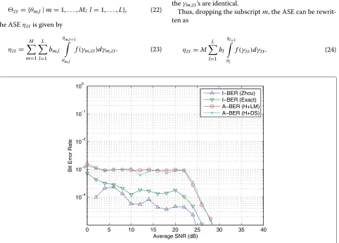
SNR thresholds for the I-BER constraint

The thresholds are obtained in the following three ways. In the first method, the thresholds are obtained from numerical search using the exact BER expressions of M-QAM in AWGN channels. In the second method, the thresholds are from (7) with constellation specific con-stants defined in . In the third method, the thresholds are also from (7) with the constants ofal=0.2 andcldefined in (6). As shown in Table 2, the second thresholds are quite close to the first, so the first and the third thresholds are used for the I-BER simulation.

SNR thresholds for the A-BER constraint

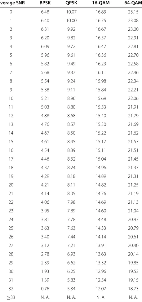
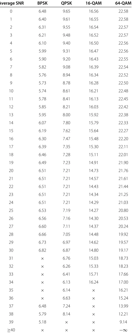
It is observed that, in (30) and (38) of Appendix, the A-BER of each MIMO mode depends on the three param-eters, M, N, and ρ. Thus, if M and N are ﬁxed, the optimal SNR thresholds change only according toρ. We obtained the optimal thresholds using a Lagrange mul-tiplier, and obtained the sub-optimal thresholds using the descending search method described in the previous section by changing ρ from 0 to 40 dB with the inter-val of 1 dB. Tables 3 and 4 show the optimal and the sub-optimal thresholds of the spatial multiplexing sys-tem with ZF receiver, and Tables 5 and 6 show those

Table 2 SNR thresholds for the I-BER constraint (δ0=10−3)

Modulation BPSK QPSK 16-QAM 64-QAM

Exact BER [14] 6.79 9.80 16.54 22.55

Huang’s method [11] 6.85 9.86 16.61 22.59

Zhou’s method [4] 7.24 10.25 17.24 23.47

Table 3 SNR thresholds for the spatial multiplexing system with ZF receiver from lagrange multiplier method

(M=N=2,δ0=10−3₎

Average SNR BPSK QPSK 16-QAM 64-QAM

0 6.48 10.07 16.83 23.15

1 6.40 10.00 16.75 23.08

2 6.31 9.92 16.67 23.00

3 6.20 9.82 16.57 22.91

4 6.09 9.72 16.47 22.81

5 5.96 9.61 16.36 22.70

6 5.82 9.49 16.23 22.58

7 5.68 9.37 16.11 22.46

8 5.54 9.24 15.98 22.34

9 5.38 9.11 15.84 22.21

10 5.21 8.96 15.69 22.06

11 5.03 8.80 15.53 21.91

12 4.88 8.68 15.40 21.79

13 4.76 8.57 15.30 21.69

14 4.67 8.50 15.22 21.62

15 4.61 8.45 15.17 21.57

16 4.54 8.39 15.11 21.51

17 4.46 8.32 15.04 21.45

18 4.37 8.24 14.96 21.37

19 4.29 8.18 14.89 21.31

20 4.21 8.11 14.82 21.25

21 4.14 8.05 14.76 21.19

22 4.06 7.98 14.69 21.13

23 3.95 7.89 14.60 21.04

24 3.81 7.78 14.48 20.93

25 3.63 7.63 14.33 20.79

26 3.40 7.44 14.14 20.61

27 3.12 7.21 13.91 20.40

28 2.78 6.93 13.63 20.14

29 2.39 6.62 13.32 19.85

30 1.93 6.25 12.96 19.53

31 1.39 5.83 12.54 19.15

32 0.76 5.34 12.07 18.73

≥33 N. A. N. A. N. A. N. A.

(6)

Table 4 SNR thresholds for the spatial multiplexing system with ZF receiver from descending search

method(M=N=2,δ0=10−3₎

0 6.48 9.65 16.56 22.58

1 6.40 9.61 16.55 22.58

2 6.31 9.55 16.54 22.57

3 6.21 9.48 16.52 22.57

4 6.10 9.40 16.50 22.56

5 5.99 9.31 16.47 22.56

6 5.90 9.20 16.43 22.55

7 5.82 9.08 16.39 22.54

8 5.76 8.94 16.34 22.52

9 5.73 8.78 16.28 22.50

10 5.74 8.61 16.21 22.48

11 5.78 8.41 16.13 22.45

12 5.85 8.21 16.03 22.42

13 5.95 8.00 15.92 22.38

14 6.07 7.80 15.79 22.33

15 6.19 7.62 15.64 22.27

16 6.30 7.47 15.48 22.20

17 6.39 7.35 15.30 22.11

18 6.46 7.28 15.11 22.01

19 6.49 7.23 14.91 21.90

20 6.51 7.21 14.73 21.76

21 6.51 7.21 14.57 21.61

22 6.51 7.21 14.43 21.44

23 6.51 7.21 14.34 21.25

24 6.51 7.21 14.29 21.03

25 6.53 7.19 14.27 20.80

26 6.56 7.16 14.30 20.53

27 6.60 7.11 14.37 20.24

28 6.66 7.05 14.48 19.92

29 6.73 6.97 14.62 19.57

30 6.82 6.87 14.80 19.17

31 _× 6.76 15.03 18.73

32 × 6.26 15.33 18.23

33 × 6.41 15.71 17.66

34 × 6.13 16.24 17.00

35 × 6.14 × 16.21

36 × 6.63 × 15.24

37 6.48 7.24 × 13.99

38 5.79 8.14 × 12.21

39 5.18 × × 9.14

≥40 × × × −∞

Table 5 SNR thresholds for OSTBC system obtained from Lagrange multiplier method (M=N=2,δ0=10−3)

0 6.36 9.96 16.72 23.04

1 6.22 9.84 16.59 22.92

2 6.03 9.67 16.42 22.76

3 5.80 9.47 16.21 22.56

4 5.56 9.26 16.00 22.36

5 5.32 9.05 15.79 22.16

6 5.03 8.80 15.53 21.91

7 4.63 8.46 15.18 21.59

8 4.17 8.08 14.79 21.21

9 4.08 8.00 14.71 21.14

10 4.26 8.15 14.86 21.29

11 4.47 8.33 15.04 21.46

12 4.57 8.41 15.13 21.54

13 4.49 8.35 15.06 21.47

14 4.19 8.09 14.80 21.23

15 3.86 7.82 14.52 20.97

16 3.81 7.78 14.48 20.93

17 3.90 7.85 14.56 21.00

18 3.96 7.90 14.61 21.05

19 3.86 7.82 14.52 20.97

20 3.49 7.51 14.21 20.68

21 2.62 6.81 13.50 20.02

22 0.19 4.90 11.67 18.37

≥23 N. A. N. A. N. A. N. A.

order modulation for the whole SNR region produces the A-BER below δ0, and also because the curve

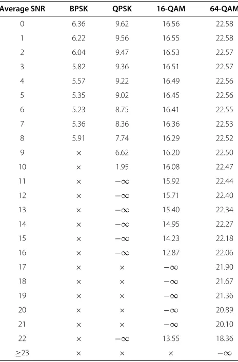
ﬁt-ting approximation of the BER is used [11]. Note that it is assumed that all the constellations are used in the optimal method. In [11], the last valid thresholds with a lower SNR is used to tackle this situation, but it causes some performance loss. Instead, in the sub-optimal method, since it is possible to switch oﬀ some constellations, the thresholds can always be obtained. Note that only 64-QAM is used for the entire instanta-neous SNR region with high average SNR as shown in Tables 4 and 6.

ASE and BER performance

(7)

Table 6 SNR thresholds for OSTBC system obtained from descending search method (M=N=2,δ0=10−3)

0 6.36 9.62 16.56 22.58

1 6.22 9.56 16.55 22.58

2 6.04 9.47 16.53 22.57

3 5.82 9.36 16.51 22.57

4 5.57 9.22 16.49 22.56

5 5.35 9.02 16.45 22.56

6 5.23 8.75 16.41 22.55

7 5.36 8.36 16.36 22.53

8 5.91 7.74 16.29 22.52

9 × 6.62 16.20 22.50

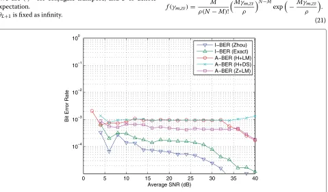
of (6) are used to get the switching thresholds for adap-tive modulation, and the Huang method means that the constellation speciﬁc constants of Table 1 are used. The A-BER approach has SNR gain of 2–3 dB compared to the I-BER method at the same ASE. In the I-BER approach, even though the exact BER function in AWGN chan-nels is used, the A-BER is still below δ0 so that it is

too conservative. In the A-BER approach, the optimal method (‘H+LM’ in the figure), in which constellation spe-cific constants defined in , and Lagrange multiplier are used, gives the best ASE performance while satisfying the A-BER constraint. In case that the constants of (6) are used (‘Z+LM’), even though Lagrange multiplier is used, gives lower performance. This means that using an accu-rate BER function in (13) is important. The sub-optimal method (‘H+DS’) also gives as good performance as the optimal method. Since the optimal thresholds are not available in high average SNR range (ZF:≥33 dB, OSTBC: ≥23 dB), the last valid thresholds are used (ZF: 32 dB, OSTBC: 22 dB) as mentioned in [11]. At low average SNR, the optimal method performs better in terms of ASE than

the optimal method. At high average SNR, the sub-optimal method is slightly better in terms of ASE than the optimal method because the search of the optimal SNR thresholds fails at high average SNR, and the last valid threshold with a lower SNR was used. Thus, we can use a hybrid scheme which uses the optimal thresholds at low average SNR, and the sub-optimal thresholds at high average SNR.

Performance of the dynamic rate-adaptive MIMO mode switching

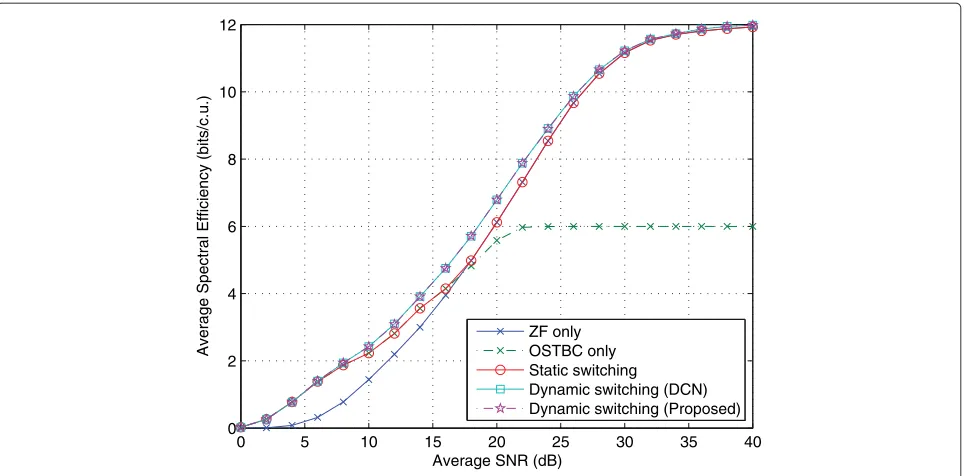
Figures 6 and 7 shows the ASE and A-BER of the proposed scheme. The SNR thresholds of the proposed scheme are obtained from the A-BER approach using the hybrid approach described in the previous section. At low aver-age SNR, the optimal thresholds are used, whereas the sub-optimal thresholds are used at high average SNR where the optimal thresholds cannot be computed (i.e., ZF: ≥33 dB, OSTBC: ≥23 dB). As shown in Figure 6, the two ASE curves that only one MIMO mode is used cross at about 17 dB. Thus, the mode switching rule of the static method is as follows: if ρ < 17, the diver-sity mode (OSTBC) is selected. Otherwise, the spatial multiplexing mode (ZF) is selected. It is observed that the proposed dynamic switching scheme has 1–2 dB SNR gain over the static switching scheme in the 10–26 dB SNR range while keeping the A-BER close to the tar-get value as shown in Figure 7. It is also observed in Figure 6 that the proposed mode switching criterion has the same performance as the Demmel condition number (DCN) method. Therefore, the proposed crite-rion is preferable in terms of computational complexity when the ISE of each MIMO mode is equal to each other.

Conclusion

(8)

0 5 10 15 20 25 30 35 40 0

2 4 6 8 10 12

Average SNR (dB)

Average Spectral Efficiency (bits/c.u.)

I−BER (Zhou) I−BER (Exact) A−BER (H+LM) A−BER (H+DS) A−BER (Z+LM)

Figure 2ASE performance of the spatial multiplexing system with ZF receiver.

Endnote

a_{In this article, we use boldface lowercase letters to denote}

vectors, boldface uppercase to denote matrices.sk is the

kth element of the vectorswhile [H]i,jis the element in theith row andjth column of the matrixH.HF is the Frobenius norm onH.

b_{We use} ₍_·₎H _{for conjugate transpose, and} _E _{to denote} expectation.

c_θL

+1is ﬁxed as inﬁnity.

Appendix: Closed form expressions of ASE and average BER for the two MIMO modes

Spatial multiplexing system with zero-forcing receiver It has been shown in [16] that the pdf of γm,ZF in (2) is

distributed as

f(γm,ZF)= M

ρ(N−M)!

_M_γm_,ZF ρ

N−M exp

− Mγm,ZF

ρ

.

(21)

0 5 10 15 20 25 30 35 40

10−4 10−3 10−2 10−1 100

Average SNR (dB)

Bit Error Rate

I−BER (Zhou) I−BER (Exact) A−BER (H+LM) A−BER (H+DS) A−BER (Z+LM)

(9)

0 5 10 15 20 25 30 35 40 0

2 4 6 8 10 12

Average SNR (dB)

Average Spectral Efficiency (bits/c.u.) I−BER (Zhou) I−BER (Exact) A−BER (H+LM) A−BER (H+DS)

Figure 4ASE performance of the OSTBC system.

Deﬁning the set of adjustable thresholdsZFas

ZF= {θm,l|m=1,. . .,M; l=1,. . .,L}, (22)

the ASEηZFis given by

ηZF=

M

m=1

L

l=1 bm,l

θm,l+1

θm,l

f(γm,ZF)dγm,ZF. (23)

Since it is assumed that channel is i.i.d., the pdf ’s of all theγm,ZF’s are identical.

Thus, dropping the subscriptm, the ASE can be rewrit-ten as

ηZF=M

L

l=1 bl

θl+1

θl

f(γZF)dγZF. (24)

0 5 10 15 20 25 30 35 40

10−4 10−3 10−2 10−1 100

Average SNR (dB)

Bit Error Rate

I−BER (Zhou) I−BER (Exact) A−BER (H+LM) A−BER (H+DS)

(10)

0 5 10 15 20 25 30 35 40 0

2 4 6 8 10 12

Average SNR (dB)

Average Spectral Efficiency (bits/c.u.)

ZF only OSTBC only Static switching

Dynamic switching (DCN) Dynamic switching (Proposed)

Figure 6ASE performance of the dynamic rate-adaptive MIMO mode switching system.

Substituting (21) into (24) and using the upper incom-plete Gamma function deﬁned as

(s,x)= ∞

x

ts−1e−tdt, (25)

ηZFcan be expressed as a closed form as follows:

ηZF= M (DZF)

L

l=1 bl

DZF,M

ρθl

−

DZF,M

ρθl+1

, (26)

whereDZF =N−M+1 and(n) =(n−1)!. Likewise,

the A-BERPe,avg,ZFcan be denoted as

Pe,avg,ZF= M

ηZF

L

l=1

blPe,ZF(l), (27)

wherePe,ZF(l)is given by

Pe,ZF(l)=

θl+1

θl

Pe(γZF,Ml)f(γZF)dγZF. (28)

0 5 10 15 20 25 30 35 40

10−4 10−3 10−2 10−1 100

Average SNR (dB)

Average BER

Static switching

Dynamic switching (DCN) Dynamic switching (Proposed)

(11)

Substituting (5) and (21) into (28), Pe,ZF(l) can be

expressed as a closed form as follows:

Pe,ZF(l)=

Substituting (26) and (29) into (27), Pe,avg,ZF is ﬁnally

obtained as

Orthogonal space-time block coding system

It is known that the pdf ofγOSTBCin (4) is distributed as [7]

f(γOSTBC)=

Since the pdf is also Gamma distributed as that of ZF case, the derivation procedure is similar. Deﬁning the set of adjustable thresholdsOSTBCas

OSTBC= {θ1,θ2,. . .,θL}, (32)

Substituting (31) into (33),ηOSTBCcan be expressed as a

closed form as follows:

ηOSTBC=

expressed as a closed form as follows:

Pe,OSTBC(l)

Substituting (34) and (37) into (35),Pe,avg,OSTBCis ﬁnally

obtained as

The authors declare that they have no competing interests.

Acknowledgements

This research was supported in part by Basic Science Research Programs (KRF-2008-314-D00287, 2010-0013397), Mid-career Researcher Program (2010-0027155) through the NRF funded by the MEST, Seoul R&BD Program (JP091007, 0423-20090051), the KETEP grant (2011T100100151), the INMAC, and BK21.

Received: 17 December 2011 Accepted: 22 June 2012 Published: 31 July 2012

References

1. GJ Foschini, Layered space-time architecture for wireless communication in a fading environment when using multiple aantennas. Bell Labs. Tech. J.1(2), 41–59 (1996)

2. SM Alamouti, A simple transmit diversity technique for wireless communications. IEEE J. Sel. Areas Commun.16(8), 1451–1458 (1998) 3. S Catreux, V Erceg, D Gesbert, RW Heath Jr., Adaptive modulation and

MIMO coding for broadband wireless data networks. IEEE Commun. Mag. 40(6), 108–115 (2002)

4. S Zhou, GB Giannakis, Adaptive modulation for multi-antenna transmissions with channel mean feedback. inProc. IEEE Int. Conf. Commun. (ICC’03)(Anchorage, USA, 2003), pp. 2281–2285

5. A Maaref, S A¨ıssa, Adaptive modulation using orthogonal STBC in MIMO Nakagami fading channels. inin Proc. IEEE Int. Symp. Spread Spectrum Tech. App. (ISSSTA’04),(Sydney, Australia, 2004), pp. 145–149

6. A Maaref, S A¨ıssa, Rate-adaptive M-QAM in MIMO diversity systems using space-time block codes. inProc. IEEE Int. Symp. Personal, Indoor and Mobile Radio Commun. (PIMRC’04),(Barcelona, Spain, 2004), pp. 2294–2298 7. Y Ko, C Tepedelenlio ˇglu, Orthogonal space-time block coded

rate-adaptive modulation with outdated feedback. IEEE Trans. Wirel. Commun.5(2), 290–295 (2006)

8. A M ¨uller, J Speidel, Adaptive modulation for MIMO spatial multiplexing systems with zero-forcing receivers in semi-correlated Rayleigh fading channels. inProc. Int. Wireless Commun. and Mobile Computing Conf. (IWCMC’06),(Vancouver, Canada, 2006), pp. 665–670

9. J Huang, S Signell, Discrete rate spectral eﬃciency improvement by scheme switching for MIMO systems. inProc. IEEE Int. Conf. Commun. (ICC’08),(Beijing, China, 2008), pp. 3998–4002

(12)

11. J Huang, S Signell, On performance of adaptive modulation in MIMO systems using orthogonal space-time block codes. IEEE Trans. Veh. Technol.58(8), 4238–4247 (2009)

12. RW Heath Jr., AJ Paulraj, Switching between diversity and multiplexing in MIMO systems. IEEE Trans. Commun.53(6), 962–968 (2005)

13. A Paulraj, R Nabar, D Gore,Introduction to Space-Time Wireless Communications(Cambridge University Press, New York, 2008) 14. MP Fitz, JP Seymour, On the bit error probability of QAM modulation. Int.

J. Wirel. Inf. Netws.1(2), 131–139 (1994)

15. P Li, D Paul, R Narasimhan, J Cioﬃ, On the distribution of SINR for the MMSE MIMO receiver and performance analysis. IEEE Trans. Inf. Theory. 52(1), 271–286 (2006)

16. D Gore, RW Heath Jr., A Paulraj, On performance of the zero forcing receiver in presence of transmit correlation. inProc. IEEE Int. Symp. Inf. Theory (ISIT’02)(Lausanne, Switzerland, 2002), p. 159

doi:10.1186/1687-1499-2012-238

Cite this article as: Kim and Lee:Dynamic rate-adaptive MIMO mode

switching between spatial multiplexing and diversity.EURASIP Journal on Wireless Communications and Networking20122012:238.