R E S E A R C H
Open Access
Structure-based learning in wireless networks
via sparse approximation
Marco Levorato
1,2*, Urbashi Mitra
1and Andrea Goldsmith
2Abstract
A novel framework for the online learning of expected cost-to-go functions characterizing wireless networks performance is proposed. The framework is based on the observation that wireless protocols induce structured and correlated behavior of the finite state machine (FSM) modeling the operations of the network. As a result, a significant dimension reduction can be achieved by projecting the cost-to-go function on a graph wavelet basis set capturing typical sub-structures in the graph associated with the FSM. Sparse approximation with random projection is then used to identify a concise set of coefficients representing the cost-to-go function in the wavelet domain. This Compressed Sensing (CS) approach enables a considerable reduction in the number of observations needed to achieve an accurate estimate of the cost-to-go function. The proposed method is characterized via stability analysis. In particular, we prove that the standard CS approach of the Least Angle Selection and Shrinkage Operator (LASSO) will not provide stability. We also determine a connection between the structure of the FSM induced by the wireless protocols and the restricted isometry property of the effective projection matrix. Simulation results of our
approximation method show that 15 wavelet functions can accurately represent a cost-to-go function defined on a state space of 2000 states. Moreover, the number of state-cost observations needed to estimate the cost-to-go function is orders of magnitude smaller than that required by traditional online learning techniques.
Introduction
Given the recent explosion in the number and types of wireless devices, new design and optimization paradigms are needed to effectively manage the complex and heterogeneous nature of modern wireless networks. We propose a novel approach for the online learning of cost-to-go functions in networks modeled via large finite state machines (FSM). Typical cost functions measure per-formance metrics such as throughput, packet delivery probability and delay. Cost-to-go functions measure the expected long-term cost incurred by the network from any state of the FSM. Estimation of cost-to-go functions is instrumental for the optimization of network con-trol strategies. Our estimation approach is based on the observation that wireless networking protocols induce a structured behavior of the FSM, enabling dimension reduction of its state space via wavelet-projection and
*Correspondence: [email protected]
1Department of Electrical Engineering, Stanford University, Stanford, CA 94305 USA
2Department of Electrical Engineering, University of Southern California, Los Angeles, USA
compressed sensing-like techniques. The sparse approx-imation approach proposed herein considerably reduces the length of the trajectory of the FSM required to achieve an accurate estimate of the cost-to-go function compared to traditional learning techniques.
Markov models have been widely used for the analysis and optimization of wireless networks [1-9]. In one of the earliest works on protocol modeling [1], a Markov chain is proposed to analyze the saturation throughput of IEEE 802.11 medium access control. The FSM models the back-off countdown counter controlling channel sensing and access of a wireless terminal and the retransmission index of the packet under transmission. In general, the Markov chains defined in these models track the logical state of the wireless protocols (e.g., the retransmission index of the packet being transmitted, the number of packets in the buffer and the backoff counter) as well as environmental variables (e.g., the channel state).
The online optimization of control strategies based on these models requires the estimation of cost-to-go functions from a sample-path of state-cost observations [10-12]. However, the immense size of the state space of FSMs associated with practical wireless networks limits
the applicability of traditional online learning techniques to toy networks and extremely simple case studies. In fact, the estimation of cost-to-go functions in traditional online learning (e.g., Q-learning and Reinforcement learning [10-12]) requires sufficient observation of a sample-path such that it hits all the states of the FSM a large number of times. Approximations of cost-to-go functions [13,14] are generally based on oversimplified models and thus cannot be accurately used in general practical networks. For instance, the fluid approximation proposed in [14] is based on the assumption that the cost-to-go function is smooth in the state space of the FSM, meaning that only small variations of its value computed in neighboring states are allowed. This assumption is suitable for sim-ple cases (e.g., buffer models and cost functions modeling buffer congestion), but does not hold for more complex FSM models and general cost functions.
This work provides the following contributions: 1) we present a framework based on CS for the approximation of cost-to-go functions; 2) we analyze the structure of the FSMs modeling wireless networks based on their decom-position into fundamental components; 3) we connect the structure of the FSM to the Restricted Isometry properties of the effective projection matrix; 4) we analyze the sta-bility of CS in this context via perturbation analysis; 5) we present a methodology for the use of Diffusion Wavelets (DW) in online learning; 6) we present numerical results illustrating the performance of the proposed approach.
The framework proposed herein is not tailored to a spe-cific canonical network example, but is rather based on the inherent structure of the FSMs modeling the operations of
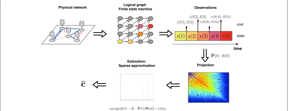
general wireless networks. The fundamental observation behind our framework is that the directed graph associ-ated with the temporal evolution of the state of the FSM is inherently regular and local. As a consequence, typical trajectories on the FSM can be described by a number of graph sub-structures considerably smaller than the num-ber of possible edges between states. Figure 1 depicts a schematic of the proposed online learning algorithm. A trajectory of the FSM associated with the operations of the physical network is used to estimate the transition probability matrix and the cost function and formulate the estimation problem. The cost-to-go function is projected onto a graph wavelet basis set capturing relevant and typi-cal substructures in the graph. Sparse approximation (and in particular the least-squares CS (LS CS) algorithm [15]) is then employed to identify a concise set of substructures to represent the cost function of interest.
We characterize the performance of sparse approxima-tion applied to the estimaapproxima-tion problem addressed herein in terms of the minimum number of states that need to be observed to achieve an accurate estimate of the cost-to-go function. Our analysis is based on the decom-position of the FSM in fundamental structures we refer to assub-chains. The transition matrix associated with the individual sub-chains is analyzed to measure the incoher-enceaof the overall transition matrix, which is exploited to determine the conditions under which the restricted isometry property (RIP) [16] holds for our effective ran-dom projection matrix.
Note that whereas most prior work on sparse approx-imation focuses on static scenarios, the framework
Figure 1Schematic of the algorithm.Graphical representation of the proposed approach. The physical network is a collection of terminals (gray circles) connected by wireless links: data (solid lines) and interference (dashed lines) links. The state of the terminals is defined by a collection of variables whose value evolves over time. The temporal evolution of the state of the terminals and of the links is modeled by the logical graph of the network. A sample-path of the network on the logical graph generates a sequence of observations, that are used to estimate the transition matrix
ˆ
considered in this article addresses the problem of learn-ing in dynamical systems. The inclusion of states visited a small number of times in the sample-path of the FSM results in instability of the estimation algorithm. To reduce this effect, we use the LS CS algorithm proposed in [15]. LS CS correlates the output of the sparse approximation algorithm by constraining variations in the support of the solution.
Relevant to the approach proposed herein, Mahadevan et al. in [17] proposed the use of DW [18] as a projection basis for the sparse approximation of cost-to-go functions. In [17], offline estimation of the cost-to-go function is considered, however, no performance analysis is under-taken. In contrast, we examine online learning and we pro-vide a detailed analysis to assess the performance of sparse approximation applied to Markov models of wireless net-works. Compressed sensing-based techniques have been previously applied to estimation problems in networks [19-24]. These works address graphs related to the physi-cal connectivity of the network, where nodes are terminals and links are specific wired or wireless links or modeled by undirected graphs. We address the fundamentally differ-ent problem of estimating functions defined on the state space of the FSM, i.e., thelogical graph of the wireless network, modeling the temporal evolution of the network from a small number of state observations.
Numerical results for a case of interest show that a small number of graph wavelets (∼15) are sufficient to accu-rately approximate a cost-to-go function defined on a state space of approximately 2000 states. Moreover, the pro-posed algorithm can estimate the cost-to-go function by observing a trajectory of the state of the FSM visiting a small subset of states in the state space.
The rest of this article is organized as follows. Section ‘System model and problem formulation’ describes the model of the network and defines the estimation problem. The sparse learning algorithm is presented in Section ‘Sparse estimation of cost func-tions’. Section ‘Structure of the graph’ proposes the decomposition of the overall graph into sub-chains and analyzes the properties of the transition probability matrix. Section ‘Perturbation analysis and performance bounds’ discusses the stability of sparse approximation applied in our context and characterizes the performance of the learning algorithm in terms of how the number of state observations grows with the network size. Numer-ical results are presented in Section ‘NumerNumer-ical results’. Section ‘Conclusions’ concludes the article. The proof of the stated theorems are in Appendices 1 and 2.
System model and problem formulation
The network is modeled as a FSM whose state evolves within the state spaceS withN = |S|. DefineS(t)∈S as
the state of the FSM at timet = 0, 1, 2,. . .. We assume that the sequenceS = {S(0),S(1),S(2),. . .} is a Markov process with transition probabilities
p(s,s)=P(S(t+1)=s|S(t)=s), (1) whereP(·)denotes the probability of an event. The per-formance of the network is measured by a functionc(s,s) that assigns a positive and bounded cost to the transition from statesto states. The average cost from statesis
c(s)=Es∈S[c(s,s)]= s∈S
p(s,s)c(s,s)b. (2)
The function
c(S(t))=c(S(t))+E
∞
τ=1
γτc(S(t+τ ))
, (3)
where E[·] denotes expectation andγ∈(0, 1) is the dis-count factor, is the expected disdis-counted long-term cost. This function is also known as thecost-to-gofunction and is central to DP and optimal control [10].
For any fixed S(t) = s∈S the function c(·) is inde-pendent of the time index t and can be rewritten as
c(s)=c(s)+
s∈S
∞
τ=1
γτpτ(s,s)c(s), (4)
where
pτ(s,s)=P(S(t+τ )=s|S(t)=s) (5) is theτ-step transition from states to s.c Consider the graph associated with the FSM, where vertices are states inSand edges are state-transitions with non-zero proba-bility. The temporal distanceτin the evolution of the FSM translates into some number of hops in the graphical rep-resentation. Starting from a vertexs,c(s)is computed by sequentially summing the discounted and weighed cost of the reachable vertices for an increasing number of hops in the graph. The representation as a graph of the temporal evolution of the network is the key for the sparse learning algorithm proposed herein.
In online learning, the function cis estimated from a sample-path of state-cost observations. The sample-path OT of observations up to timeT includes the sequence of states {S(0),S(1),. . .,S(T)} and state transition costs {c(S(0),S(1)),. . .,c(S(T−1),S(T))}. Denote bycthe vec-tor collecting the expected long-term costc(s)for alls∈S, i.e.,c=[c(1),c(2),. . .,c(N)].dThe objective is to build an estimator ofcbased on the observationsOTminimizing a distance metric such asˆcT−c22, wherecˆTis the estimate at timeT.
spaceS underlying the associated FSM. In fact, in tradi-tional online learning an accurate estimation ofcrequires a sample-path of observations where each state in S is visited a considerable number of times. In fact, all the allowed state transitions need to be observed a sufficient number of times to estimate their probability.
Sparse estimation of cost functions
We now present an algorithm for the online learning of cost-to-go functions in wireless networks from the obser-vation of a state-cost trajectory of the associated FSM. The baseline observation is that networking protocols induce a structured behavior of the network, which is reflected in a structured graph associated with the FSM. Thus, every state-cost observation conveys information about multi-ple states due to the correlated behavior of the network. As a result, we can propose an algorithm to estimate c exploiting this structure from fewer observations than in traditional learning. The algorithm is composed of three elements:
• observation:the transition probabilities and cost functionc(·)are estimated by observing a state-cost sample-path;
• projection: cis projected onto a graph wavelet basis set capturing typical structures in the graph;
• sparse estimation of c:a sparse estimation algorithm is used to identify a concise set of basis functions providing the best fit with the estimated transition probabilities and cost function.
We define theN×NmatrixPto be the probability tran-sition matrix whereP[s,s]=p(s,s)as in Equation (1).
The long-term costccan be rewritten as
c=c+ ∞
τ=1
γτPτc=c+γP c. (6)
Thus, c can be computed as the fixed point solution c = (c)of the operator(c) = c+γP c. The transi-tion matrixP and cost vectorcare not known a priori and need to be estimated from observation. At timeT, the sample-pathOT is used to compute the estimatesPˆ(T) andcˆ(T)ofPandc. We use the estimator
where1(·)is the indicator function. More refined estima-tors can be employed to reduce the sampling rate [25].
The estimates Pˆ(T) and cˆ(T) may be very noisy and incomplete estimates of P and c even for TN. In fact, an accurate estimation of the transition probabili-ties from a state s in S and the cost function c(s) may require a considerable number of visits tos. For asymp-totically large T, the average number of times the FSM is in state s is Tπ(s), where π(s) = limt→∞P(S(t) = s|S(0) = s0) is the steady-state probability of s. Note that the average steady-state probability of the states in S is 1/N, and thus the average number of visits to a state is T/N. However, in a finite-length sample-path, the trajectory of the state of the FSM may remain confined in a region of S even for lengths T larger than N and the number of states visited may be much smaller than T. Thus, due to the large size of the state space of FSMs modeling wireless networks, the number of observations needed to achieve an accurate estimation of the cost-to-go function is generally enor-mous, and it may be larger than the coherence time of the network, meaning that the statistics of the stochas-tic process modeling the operation of the network may change before the learning process achieves a meaningful estimate ofc.
A fundamental element of the proposed framework is the projection of the cost-to-go function c on a set of basis functions capturing the typical substructures of the graph at various time scales. In fact, every new observa-tion updates the estimate of all the substructures including the observed transition. We employ the recently proposed DWs [18] as a basis set for the projection. DWs are a multiresolution geometric construction for the multiscale analysis of operators on graphs. DW functions are com-puted by sequentially applying a diffusion operator (for instance, the transition matrix P) at the current scale k, compressing the range via a local orthonormalization procedure, representing the operator in the compressed range and computing the P2k on this range. Functions defined on the support space are analyzed in multires-olution fashion, where dyadic powers of the diffusion operator correspond to dilations, and projections corre-spond to downsampling. Even ifPis not knowna priori, we assume that the location of the non-zero elements ofP, that is, the connectivity structure ofP, is knowne. Define I(P)=sgn(P+PT). The basis set W is then computed on Psymmwhere theith row ofPsymmis
[Psymm]i=[I(P)]i/
j
[I(P)]ij. (9)
The symmetrization step is required as DWs presume symmetric diffusion operators. The design of wavelet functions tailored to the compression of directed graphs will further improve the performance of the algorithm proposed herein.
DefineWas a diffusion wavelet basis set computed on Psymm, where the DW functions are the columns ofW. We have thenc˜≈Wx, wherexis the representation vec-tor collecting the coefficients of the wavelet functions in W. GivenPandc, the representation vectorx∗providing the most accurate approximation ofconWminimizes the Bellman residual(Wx)−Wx22. We have then
x∗=arg min
x c−(I−γP)Wx
2
2. (10)
The main idea behind the estimation paradigm pro-posed herein is that the DW set of functions is a sparsifying basis for the cost-to-go function c. Due to the structured behavior defined by networking protocols, a small number of functions can represent the evolu-tion and, thus, the collected cost, from large groups of states. The Least Angle Selection and Shrinkage Operator (LASSO) algorithm [26] minimizes the residual norm of the residual plus a regularization term. For the considered problem, the LASSO is formulated as
x∗(T)=arg min
x R(T)cˆ(T)−R(T)Bˆ(T)Wx
2
2+λx1,
(11)
whereBˆ(T)= R(T)(I−γPˆ(T))andR(T)is a random projection matrix. The-1 regularization termλx1 is a sparsity-promoting term, meaning that the least signifi-cant coefficients inxare pushed toward zero.
In the Compressed Sensing (CS) literature, the matrix ˆ
B(T)andWin the above equation are generally referred to as thesensingandrepresentationmatrices, respectively. Note that the elements in the rows ofPˆ(T)andcˆ(T) cor-responding to states not visited in the trajectoryOT are set to zero and can be eliminated in the projection.
Structure of the graph
Wireless networking protocols induce a very structured temporal evolution of the network, and, thus, a very struc-tured graph associated with the FSM. This structure is the key to show some general properties of the transition matrixPthat determines the performance of the sparse reconstruction in terms of the minimum number of states that needs to be included in Equation (11) to achieve an accurate reconstruction. Our analysis is based on the decomposition of the overall graph into smaller graphs, which we refer to as sub-chains. The good incoherence properties of the transition matrices associated with the sub-chains are reflected in good incoherence of the over-all transition matrix and, thus, result in good performance of the sparse reconstruction.
The decomposition into sub-chains of the complex graph associated with the FSM modeling the temporal evolution of wireless networks results from the obser-vation that the state of the network is the collection of many individual descriptors tracking counters and vari-ables associated with the functioning of protocols and the environment. The temporal evolution of each individual descriptor follows simple rules that can be easily analyzed to retrieve properties of the overall graph. We then define S(t) = {S1(t),. . .,SD(t)}, whereSd(t) is the state of the dth sub-chain at timet. We denote bySd the state space of thedth sub-chain, with|Sd| =Nd.
The sub-chains track the evolution of the individual components of the state space. Although in the overall FSM the transition probabilities are a function of the over-all state of the network,the connectivity structure of the sub-chains is preserved in the overall FSM. In fact, the state transition froms= {s1,. . .,sD}∈Stos = {s1,. . .,sD}∈S in the overall FSM is allowedf only if the state transition fromsd tosd is allowed in the corresponding sub-chain, for alld=1,. . .,D. Thus, the properties of the connectiv-ity structure of the sub-chains are inherited by the overall graph.
In stochastic models for wireless networks two classes of sub-chains can be identified:
b
c
a
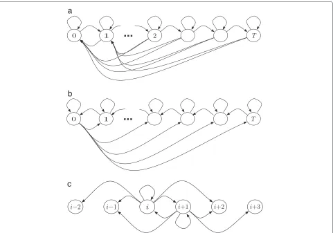
Figure 2Sub-chains.(a)Counter-like sub-chain, forward counter.(b)Counter-like sub-chain, backward counter.(c)Random walk sub-chain.
increments/decrements until it is reset to a given value. Examples of counter-like sub-chains are: the number of retransmissions of a packet in ARQ protocols, the backoff timers in DCF and the transmission windows and timers in TCP. This class can be further divided into forward counters (Figure 2a and backward counters (Figure 2b, depending on whether the counter is incremented or decremented until being reset to a predefined value;
• Random walk sub-chains(see, Figure 2c): the value of the descriptor variable is subject to random, but constrained, increments and decrements. Examples of random walk sub-chains are channel state descriptors and variables tracking the number of packets in a buffer.
For instance, in the pioneering work [1], the Markov chain used to analyze the network is the composition of a random walk and a counter-like sub-chain. It can be observed that counter-like and random walk sub-chains present a very local and regular connectivity structure. By local, we mean that every state connects to a small neigh-borhood of states. Regularity implies that states connect
to 1-hop neighbors in a similar fashion. For instance, in counter-like sub-chains, states connect to the state cor-responding to a reset counter and the state associated with an incremented or decremented value (possibly plus a self-loop). As a result, the overall graph is regular and local. This property is instrumental towards having an efficient compression in the wavelet domain, meaning that only a limited number of notable substructures is needed to model the temporal evolution of the state of the network.
few particular states whose effect decreases as the dimen-sion of the Markov chain increases, given two states id,jd∈{1,. . .,nd}, with id=jd, the number of states in S←
d (id)∩Sd←(jd) is generally small and so is the inner productNd
kd=1pd(kd,id)pd(kd,jd). Since the connectivity
structure of the overall graph results from the composi-tion of the connectivity structures of the sub-chains, the inner product of the columns ofPis intuitively small. In order to perform a quantitative analysis of the inner prod-ucts ofP, we focus on the natural random walk defined on the sub-chainsg, that is we assign equal probability to all the allowed transitions from a given state. We have, then,
pd(id,jd)=1/|Sd→(id)|, ∀id∈Sd, ∀jd∈Sd→(id), (12) wherepd(id,jd)is the transition probability from stateid andjd in the state space of thedth sub-chain. Then, the inner product between theith and thejth columns ofPis
N the states associated with statesi,j, andk, respectively.
We then need to compute the inner products of the columns of the transition matrices associated with the classes of sub-chains. The average inner products of the backward counter, forward counter and random walk sub-chains are, respectively,
where in a random walk sub-chain the transition prob-ability from state id to state jd is larger than zero only if|jd−id|≤and we assumeNd2+1. We observe that all these mean inner products are of order O(N1
d). As
an example of how these quantities are computed, con-sider the forward counter-like sub-chain. The associated transition matrix is
We remark that the value of the transition probabil-ity pd(id,jd) is the inverse of the number of outgoing links, i.e., allowed transitions, fromid. The average inner
productEid,jd
sequentially considering all the columns indexed byid = 1,. . .,Nd−1 and computing the product with the columns indexed byjd>id.
The average inner products of the sub-chains decrease on average with the number of states of the associated FSM. Although in the general case the probability of tran-sition from a state to its neighbors may be much different from that provided by the natural random walk associ-ated with the graph structure, the locality and regularity of the structure of the sub-chains cause the average overlap of the setsSd←(jd) to vanish asNd increases. Thus, suf-ficiently large sub-chains are associated with incoherent transition matrices.
The average inner product of a column with itself is also relevant to the performance of the sparse reconstruction (these means appear in the mean of the Gram matrix in the effective random projection). It is easy to compute that the average of this quantity for the counter-like backward sub-chain, counter-like forward sub-chain and random walk sub-chain is
whereCis a positive constant smaller than 1. We observe that each of these means can be expressed asO(N1
d)+αd,
Perturbation analysis and performance bounds In this section, we characterize the performance of the sparse approximation of the cost-to-go function proposed herein. We first discuss the stability of the solution of (11) and then determine how much compression is possible to ensure good reconstruction of the value function v. The number of observations required for good recon-struction directly translates to the learning rate of our proposed algorithm. An exact analysis of the transition matrix is challenging; however, by exploiting the average behavior of several key structures, we can determine the relationship between the minimum number of observa-tions for this compressed sensing problem and the size of the logical graph.
Perturbation analysis
We discuss in this section how estimation noise in the sensing matrixBˆ(T) = (I−γPˆ(T))affects the stability of the reconstruction provided by (11) as new states are visited by the sample-path. We show that the inclusion in (11) of a row incˆ(T)andPˆ(T)associated with a state hit by the FSM a small number of times may result in a dramatic change ofx∗(T)with respect tox∗(T −1). As we are looking for the fixed point solution of the opera-tor, instability and large variations of the sparse solution are highly undesirable. In order to improve the stability of the algorithm, in the numerical results presented in Section ‘Numerical results’ we use the LS CS algorithm proposed in [15].
Define ˆ
A(T)= ˆB(T)W=(I−γPˆ)(T)W. (21)
In [27], Xu et al. have shown that the regularized regres-sion problem of LASSO:
min
x ˆc(T)− ˆA(T)x
2
2+λx1 (22)
is equivalent to the robust regression (RR) problem, stated as drop the dependence onT of the estimated matrices and vectors. Thus, the vectorxis optimized for a worst case perturbation whose range is determined by the param-eter λ, that is, the algorithm is robust to perturbations. Interestingly, the larger the value ofλ, the sparser the out-put vectorx, but also the larger the set of perturbations considered. In [27], it was also shown that LASSO is not stable, meaning that small variations of the sensing matrix
ˆ
Amay lead to significantly different output vectors.
The following addresses the instability issues in the solu-tion to the RR problem. In particular, the theorem shows that the inclusion of a new sample may result in sub-optimal solutions to the RR problem. Moreover, due to the equivalence between LASSO and the RR problem, the same instability result applies to LASSO as well.
Theorem 1. Letx∗be the solution of the problem
min
of LASSO changes if a new state meeting the hypothesis is added to the Bellman residual.
The proof of the theorem is in Appendix 1.
Minimum number of observations
In Section ‘Numerical results’, we will employ the LS CS residual algorithm [15] to minimize the Bellman residual subject to a sparsity constraint:
(v)−v22= c−(I−γP)Wx22h. (28) We will observe the temporal evolution of the Markov Chain over multiple time-steps, as such, we will not observe the cost at every state. Thus, coupled with addi-tional random mixing to exploit the benefits of com-pressed sensing, we will optimize the following modified Bellman residual:
number of non-zero components and the noise variance. Comparable analysis can be made for LASSO [29,30]. We focus on properties ofR(T)(I−γP)recognizing that pro-jecting onto an orthonormal W would be an isometric operation. We note that a negative result regarding RIP would call the use of our approach into question. How-ever, a positive RIP result suggests that our method work. Analysis of LS CS also relies on RIP parameters.
Our proof exploits arguments from [31] with appro-priate tailoring to our framework. We begin with the definition of the properties we wish to show.
Definition 1. (Restricted Isometry Property): The obser-vation matrixBis said to satisfy therestricted isometry propertyof order S ∈ Nwith parameterδS ∈ (0, 1),i.e. RIP(S,δS)if
(1−δS)x22≤ Bx22≤(1+δS)x22, (30)
holds for all x∈RN having no more than S non-zero entries. Note thatBis a K×N matrix. RIP implies thatB is approximately an isometry for S-sparse signals.
We have the following result,
Theorem 2. The matrix RH(I − γP) does not satisfy RIP(S,δS) with the following probability bound,
PRHBdoes not satisfy RIP(δS,S)
≤ exp
−c1K
S2
if K2 ≥ 192 lognS2
δS2−64c1 and c1 ≥ δ2S
64. The matrix P is the transition probability matrix for a Markov chain formed by concatenating forward and backward counter-like and random walk sub-chains andγ <1. The proof of Theorem 2 can be found in Appendix 2.
We observe that this result states that if the number of observations K is of orderO
S2nlogn
then RIP
is satisfied with high probability as the network grows large. We contrast this with the more typical results seen in say channel estimation problems where the order is OS2logn. We remark that our result on the RIP is not limited to LASSO, but leads to the more general con-clusion that sparse estimation algorithms can be used to approximate cost-to-go functions of wireless networks. Furthermore, the proof of Theorem 2 shows that an arbi-trary concatenation of sub-chains does not affect the RIP property in the limit of large wireless networks.
Numerical results
In this section, we present numerical results for an exam-ple of a wireless network to demonstrate the potential of the compressed sensing approach. We consider a wire-less network where terminals store packets in a finite buffer of size Q and employ Automatic Retransmission reQuest (ARQ) to improve the delivery rate of pack-ets. Time is divided in slots of fixed duration. For the sake of simplicity we assume that the transmission of a packet occurs in the duration of a time slot and that channel coefficients in the various slots are i.i.d.. Ter-minals with a non-empty buffer access the channel in a time slot with fixed probability equal to α. The fail-ure probability of a packet transmitted by a terminal is a function of the set of terminals concurrently transmit-ting in the same slot. Packet arrival in the buffer of the terminals is modeled according to a Poisson process of intensityσ.
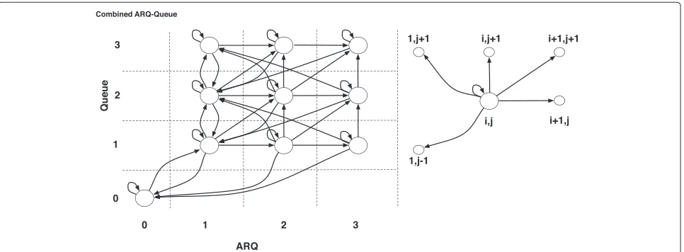
The FSM tracking the state of each individual terminal (see Figure 3) is composed of two sub-chains: a random walk-like sub-chain tracking the number of packets in the buffer (state space {0, 1,. . .,Q}) and a forward counter-like sub-chain tracking the retransmission index of the
Figure 3Example of composition of sub-chains.FSM of a terminal in the considered network: a forward-counter sub-chain (packet
Figure 4Value function and its approximation.Value function (green) and its approximation (blue).
packet being transmitted (state space{0, 1,. . .,F}, where Fis the maximum number of transmissions of a packet). An additional binary variable is added to the FSM to track transmission/idleness of the terminal. The FSM track-ing the state of the overall network is the composition of the FSMs of the individual terminals. The transition probabilities of the Markov process determining the tra-jectory of the state of the network in the state space of the FSM are a function of the packet arrival rate, of the failure probability function and of the transmission probabilityα.
The cost function c measures the normalized cost in terms of throughput loss with respect to the saturation throughput achieved by the terminals in the absence of interference. In particular, the cost function is defined as
the sum for all the terminals of one minus the failure prob-ability of the transmitted packets. Idleness is assigned a cost equal to 1.
ForQ=5 andF=4 and 2 terminals the size of the state space is 1681. The transition matrixPis used to compute Psymm defined in Equation (9) and the associated set of DW functions W[18]. DW basis sets are overcomplete. In order to keep complexity low, the columns of Ware subsampled. In particular, we select 400 wavelet functions at different time scales.
Figure 4 and 5 depict the exact and reconstructed value function using LASSO mapped on the state-action space and the sorted magnitude of the coefficients x∗, respectively. In these figures, the exact vector c and
transition matrix P are used in order to show the
properties of the sparse reconstruction based on DW. An accurate approximation ofcis achieved with approx-imately 15 active coefficients in x. This result shows that the temporal evolution of complex wireless net-works can be effectively represented by a small number of wavelet function capturing typical substructures in the graph.
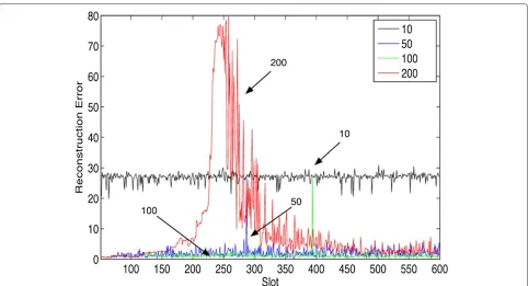
Figure 6 plots the reconstruction error (norm-2 of dif-ference between the real and reconstructed value func-tions weighted by the steady-state distribution) as a function ofT achieved by LASSO for different values of the sampling rates. The estimated transition probability matrixPˆandcˆare used for the estimation ofc. States are sampled by randomly eliminating rows (among the states visited by the sample path) of the cost vectorcˆand transi-tion matrixP. In the legend, the maximum number statesˆ included in the Bellman residual is reported. As expected, if only a few states are included in the estimation, LASSO achieves very poor performance irrespectively of the accu-racy in the estimates of the cost vector and transition matrix. However, if all the states are included in the Bell-man residual, then poorly estimated states introduce rows affected by large noise both in Pˆ and c. As shown inˆ Section Perturbation analysis, noisy rows ofPmay desta-bilize the support ofxand lead to poor reconstruction. However, the performance of LASSO is very sensitive to the sampling rate and it is unclear how to compute its optimal value.
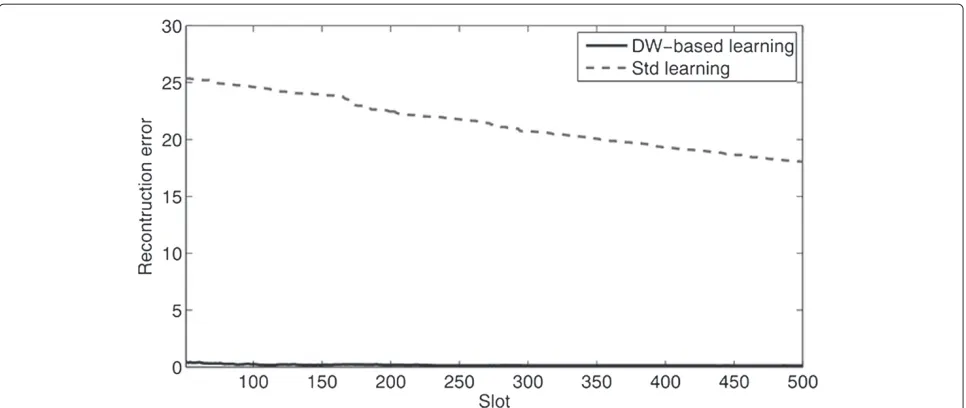
Figure 7 depicts the reconstruction error achieved by the LS CS-based framework and that of standard Q-learning [10] as a function of the length of the observed
sample-path. All states visited by the process are included in the Bellman residual. In order to improve stabil-ity, to generate this plot we used the LS CS algorithm. LS CS correlates x∗(T) to x∗(T − 1) by constrain-ing changes in the support of the representation vec-tor. Interested readers are referred to [15] for a detailed description and performance characterization of the algorithm.
The proposed algorithm achieves a considerable accu-racy in the estimation ofcafter a very short number of state-cost observations, whereas standard learning con-verges slowly to c. Moreover, the solution is extremely stableand the LS CS-based algorithm appears to be very robust to estimation noise.
Conclusions
A novel framework for the online estimation of cost-to-go functions in wireless networks was proposed. We showed that the inherent regular and local structure of the graph associated with the FSM modeling the oper-ations of wireless networks enables the sparse repre-sentation of cost-to-go functions. Our analysis, based on the decomposition of the overall graph in funda-mental smaller structures, connects the structure of the FSM to the RIP of the transition probability matrix. Numerical results show that sparse approximation and projection onto DW basis sets enable a considerable reduction in the number of observations needed to estimate cost-to-go functions in wireless networks, and have the potential to make online learning practical in this context.
Figure 7Reconstruction error as a function of time.Comparison between the reconstruction error as a function of the time slot achieved by the proposed algorithm and Q-learning. All states visited by the sample path are used in the estimation.
Endnotes
aThe incoherence of the transition matrix is connected to
the magnitude of the inner products of its columns. bNote that c(s,s) can be generalized to be a random
variable. In this case the expectation is over all the possible values ofc(s,s).
cControl can be included in the model by defining
statistics and cost functions conditioned on a control action.
dThe indexing in the vector is based on a univocal map
betweenSand{1, 2, 3,. . .,N}.
eNote that this assumption does not reduce the
applica-bility of the proposed algorithm. In fact, the connectivity structure of the transition matrix is determined by stan-dard protocols that are shared and known by all the nodes.
fBy allowed, we means that the state transition has
probability equal to zero for any set of parameters. gWe note that numerical evaluations of incoherence for
many typical Markov chains has revealed that incoherence holds on average.
hIn this analysis we assume that W is an
orthonor-mal set of basis functions. We are aware that DW are overcomplete and, thus,W is not an orthonormal basis set. The design of orthonormal wavelet basis tailored to FSMs modeling wireless networks is an important research direction.
Appendix 1
Proof of Theorem 1
Fix the indexkin the supportIx∗ofx∗, define
ˆ ai=
ˆ ai ˆ ai
,i=1,. . .,m, (31)
and the vector
u=
u u
∈spanaˆi,i∈Ix∗\k,cˆ
, (32)
withu2=1 and
ˆ c=
ˆ c b
. (33)
If
λ≥max j/∈Ix∗
|aj| (34)
and
max
u
uTaˆ
k ≤λ+λ (35)
then uT aˆ
j = |uaˆj+uaˆj| (36)
≤ √uaˆj uTu
uTu+ |uaˆ
j| (37)
≤ uTuλ+ |uaˆ
Therefore, if the conditions (34) and (35) hold, then due to
Then, we finduthat maximizes the left-hand side of (35) as the solution of
LetM= QSZbe the singular value decomposition ofM, then (41) is equal to
max
and using the Schwarz inequality we obtain
|˜dTSTa˜|2
where the equality holds ifd˜ =g. Therefore,
max
In this appendix, we prove the result on the minimum number of observed states needed for perfect reconstruc-tion ofc. We first state the following lemma:
Lemma 1. (Gerˇsgorin) The eigenvalues of an m×m matrix G all lie in the union of the n discs di = di(ci,ri),i =
We will apply Gersgorin’s lemma to the following Gram matrix,
G=(I−γP)TRT(T)R(T) (I−γP). (50)
For the sake of exposition we assume thatR(T)is anK×n matrix whose components are drawni.i.d.from a binary
distributioni.e.Rik = ±
! 1
K with probability 12; thus we have that theR(T)ik are zero mean andERTHR(T)= I. Other properly constrained distributions forR(T)can be handled. The other matrices specified in (50) are square and of dimensionn×n.
We shall show that every element of the Gram matrix, Gis bounded as follows, wheremij=EGij,
|Gii−mii| ≤d, Gij−mij ≤
o
S i=j (51)
The dimension of the state-space,|S| =. N is approxi-mately"dnd, thus from the analysis of the inner prod-ucts/norms of columns of the transition matrix (see Equations (14)–(16)) we find thatE
pTi pj
≈ON1,i=j andEpi2 ≈ ON1+αD, where pi is the ith col-umn ofP. We note that for all three sub-chain structures examinedα <1 and thus limD→∞αD = 0. In fact, if we concatenate several sub-chains we have that E[pi2]≈ O(1/N)+"Dd=1αd, where|αd|<1. Thus,E[pi2] dimin-ishes, and eventually vandimin-ishes, as the number of concate-nated sub-chains increases. Additionally, EPij
= 1
n. Thus we can show that,
assumptions onR. For clarity, we have dropped the
sub-, and observe from the statement of McDiarmid’s inequalities that we need to evaluate
The same bound holds for the off-diagonal elements of the Gram matrix. Using these values of cl0,j0 we invoke McDiarmid’s inequality to show the following, wherein (a) and (b) follow from union bound arguments and (c) follows from settingo=d= δ2S
Equation (60) can be manipulated to yield the follow-ing relationship between the number of samples K and the size of the logical network,n: the RIP holds with high probability ifK2≥ 192 lognS2
δ2S−64c1 , wherec1is constant selected to ensure that the denominator of the previous expression is positive and the Theorem is shown.
Competing interests
The authors declare that they have no competing interests.
Acknowledgements
The study was supported by AFOSR under grants FA9550-08-0480 and FA9550-12-1-0215 and by the National Science Foundation (NSF) under Grant CCF-0917343.
Competing interests
The authors declare that they have no competing interests.
Received: 16 February 2012 Accepted: 18 July 2012 Published: 30 August 2012
References
1. G Bianchi, Performance analysis of the IEEE 802.11 distributed coordination function. IEEE J. Sel. Areas Commun.18(3), 535–547 (2000) 2. A Konrad, B Zhao, A Joseph, R Ludwig, A Markov-based channel model
algorithm for wireless networks. Wirel. Netw.9(3), 189–199 (2003) 3. H Wu, Y Peng, K Long, S Cheng, J Ma, inproceedings of IEEE Twenty-First
Annual Joint Conference of the IEEE Computer and Communications Societies, INFOCOM 2002. Performance of reliable transport protocol over, IEEE 802.11 wireless, LAN analysis and enhancement, (New York, USA, 2002), pp. 599–607. vol. 2, June 23–27
4. M Zorzi, RR Rao, On the use of renewal theory in the analysis of ARQ protocols. IEEE Trans. Commun.44(9), 1077–1081 (1996)
5. L Badia, M Levorato, M Zorzi, Markov analysis of selective repeat type II hybrid ARQ using block codes. IEEE Trans. Commun.56(9), 1434–1441 (2008)
6. E Modiano, An adaptive algorithm for optimizing the packet size used in wireless ARQ protocols. Wirel. Netw.5(4), 279–286 (1999)
7. H Zhai, Y Kwon, Y Fang, Performance analysis of IEEE 802.11 MAC protocols in wireless LANs. Wirel. Commun. Mob. Comput.4(8), 917–931 (2004) 8. H Su, X Zhang, Cross-layer based opportunistic MAC protocols for QoS
provisionings over cognitive radio wireless networks. IEEE J. Sel. Areas Commun.26, 118–129 (2008)
9. M Dianati, X Ling, K Naik, X Shen, A node-cooperative ARQ scheme for wireless ad hoc networks. IEEE Trans. Veh. Technol.55(3), 1032–1044 (2006)
10. DP Bertsekas,Dynamic Programming and Optimal Control, 2nd edn., vol. 2. (Athena Scientific, Belmont, MA,2001)
11. S Mahadevan, Average reward reinforcement learning: Foundations, algorithms, and empirical results. Mach. Learn.22, 159–195 (1996) 12. A Schwartz, inProceedings of the Tenth International Conference on Machine Learning. A reinforcement learning method for maximizing undiscounted rewards, (Amherst, Massachusett, 1993), p. 305. vol. 298 13. F Fu, MVD Schaar, inArXiv preprint. Structure-aware stocastic control for
transmission technology, (2010). arXiv:1003.2471
14. W Chen, D Huang, A Kulkarni, J Unnikrishnan, Q Zhu, P Mehta, S Meyn, A Wierman, inProceedings of the 48th IEEE Conference on Decision and Control. Approximate dynamic programming using fluid and diffusion approximations with applications to power management, (Shangai, China, 2009), pp. 3575–3580. Dec. 16-18, 2009
15. N Vaswani, LS-CS-residual (LS-CS): compressive sensing on least squares residual. IEEE Trans. Signal Process.58(8), 4108–4120 (2010)
16. E Candes, MB Wakin, An introduction to compressive sampling. IEEE Signal Process. Mag.25(2), 21–30 (2008)
17. M Maggioni, S Mahadevan, A multiscale framework for Markov decision processes using diffusion wavelets. Technical report, Department of Computer Science, University of Massachusetts, 2006. [http://citeseerx.ist. psu.edu/viewdoc/download?doi=10.1.1.74.8956&rep=rep1&type=pdf] 18. RR Coifman, M Maggioni, Diffusion wavelets. Appl. Comput. Harmonic
Anal.21, 53–94 (2006)
19. M Crovella, E Kolaczyk, inINFOCOM 2003 Twenty-Second Annual Joint Conference of the IEEE Computer and Communications. Graph wavelets for spatial traffic analysis, (San Francisco, CA, USA, 2003), pp. 1848–1857. vol. 3, Mar. 30–Apr. 3
20. M Firooz, S Roy, inproc. of IEEE Global Telecommunications Conference (GLOBECOM). Network tomography via compressed sensing, (Miami, Florida, USA, 2010), pp. 1–5. Dec. 6-10
22. J Haupt, WU Bajwa, M Rabbat, R Nowak, Compressed sensing for networked data. IEEE Signal Process. Mag.25(2), 92–101 (2008) 23. M Wang, W Xu, E Mallada, A Tang, Sparse recovery with graph constraints:
fundamental limits and measurement construction. Arxiv preprint arXiv:1108.0443 (2011)to appear in Proceedings of IEEE INFOCOM 2012 24. W Xu, E Mallada, A Tang, inProceedings of the 30th IEEE International
Conference on Computer Communications (IEEE INFOCOM). Compressive sensing over graphs, (Shangai, China, IEEE, 2011), pp. 2087–2095. Apr. 10-15
25. C Sherlaw-Johnson, S Gallivan, J Burridge, Estimating a Markov transition matrix from observational data. J. Operat. Res. Soc.46(3), 405–410 (1995) 26. R Tibshirani, Regression shrinkage and selection via the Lasso. J. Royal
Stat. Soc. Ser. B.58, 267–288 (1996)
27. H Xu, C Caramanis, S Mannor, Robust regression and Lasso. IEEE Trans. Inf. Theory.56(7), 3561–3574 (2010)
28. E Candes, T Tao, The dantzig selector: statistical estimation whenpis much larger thann. Annals Stat.35(6), 2313–2351 (2007)
29. CH Zhang, J Huang, The sparsity and bias of the Lasso selection in high-dimensional linear regression. Annals Stat.36(4), 1567–1594 (2008) 30. T Zhang, Some sharp performance bounds for least squares regression
with L1 regularization. Annals Stat.37(5A), 2109–2144 (2009)
31. J Haupt, W Bajwa, G Raz, R Nowak, Toeplitz compressed sensing matrices with applications to sparse channel estimation. IEEE Trans. Inf. Theory. 56(11), 5862–5875 (2010)
doi:10.1186/1687-1499-2012-278
Cite this article as:Levoratoet al.:Structure-based learning in wireless net-works via sparse approximation.EURASIP Journal on Wireless Communications and Networking20122012:278.
Submit your manuscript to a
journal and benefi t from:
7Convenient online submission 7Rigorous peer review
7Immediate publication on acceptance 7Open access: articles freely available online 7High visibility within the fi eld
7Retaining the copyright to your article