R E S E A R C H
Open Access
Dynamics of a class of neutral three neurons
network with delay
Ming Liu, Chunrui Zhang
*and Xiaofeng Xu
*Correspondence:
[email protected] Department of mathematics, Northeast Forestry University, Harbin, 150040, P.R. China
Abstract
In this paper, a class of neutral neural networks with delays is investigated. The linear stability of the model is studied. It is found that a Hopf bifurcation also occurs when some delays pass through a sequence of critical values. The direction of the Hopf bifurcations and the stability of bifurcating periodic solutions are determined by using the normal form method and center manifold theory. The existence of a permanent oscillation is established using Chafee’s criterion. Numerical simulations are performed to support the analytical results.
Keywords: neutral neural network; stability; Hopf bifurcation; permanent oscillation
1 Introduction
Since s, the theories and applications of neural networks with delays have been greatly developed. It is well known that many important mathematical models from physics, bi-ology,etc.can be written in neurons network models. In , Li and Yuan considered a Hopfield-type network of three identical neurons coupled in any possible way in []:
˙
Due to the finite speed of the switching and transmission of signals, neutral behavior does exist in the neural network with delays and should be incorporated. For this reason, we improve the original model in which the neutral behavior was added and obtain the fol-lowing forms []:
whereaij,bij(i=j,i,j= , , ) have the values or , depending whether the cells from
j to i are connected or not;a,b,a,b∈Rdenote the strength in self-connection and neighboring-connection, respectively;τs,τn≥ are the corresponding time delays.
Fur-thermore,f,g,f, g are assumed to be adequately smooth and to satisfy the following conditions:
(H) f() =g() =f() =g() = ,
(H) f() =g() =f() =g() = .
(.)
Then we derive the stability of this system and conditions of existence of the bifurca-tion witha=a=a=a= ,a=a= ;b=b=b=b= ,b=b = , τs=τn=τ. The remainder of this paper is organized as follows. In Section we introduce
the stability of the equilibrium point and the conditions of existence of a local Hopf bifur-cation. We are devoted to establishing the direction and stability of the Hopf bifurcation in Section . In Section we discuss the existence of a permanent oscillation. Finally, we carry out some numerical simulation to support the analysis result in Section .
2 Stability and Hopf bifurcation analysis
In this section, we leta=a=a=a= ,a=a= ;b=b=b=b= ,b=
b= , then we have
˙
x(t) = –x(t) +afx(t–τ)+bgx(t–τ)+bgx(t–τ)
+af
˙
x(t–τ)
+bg
˙
x(t–τ)
+bg
˙
x(t–τ)
,
˙
x(t) = –x(t) +afx(t–τ)+bgx(t–τ)
+af
˙
x(t–τ)+bg
˙
x(t–τ), ˙
x(t) = –x(t) +bgx(t–τ)+afx(t–τ)
+bg
˙
x(t–τ)+af
˙
x(t–τ).
(.)
Under the given hypotheses (H) and (H), it is easy to check thatx= (, , )Tis an equi-librium point of system (.). By using a similar method to that in [], we have the following results on stability to system (.).
Theorem Let|a+b|< and|a–b|< .
() If(a,b)∈D,then the zero solution of system(.)is absolutely stable. () If(a,b)∈D,then the zero solution of system(.)is conditionally stable,i.e.,
τ∈[,τ),the zero solution of system(.)is asymptotically stable;τ>τ,the zero solution of system(.)is unstable,
(a) ifa< –,system(.)undergoes a Hopf bifurcation at the origin whenτ=τj, j= , , , . . .,
(b) ifa+b< –,system(.)undergoes a Hopf bifurcation at the origin whenτ=τj, j= , , , . . .,
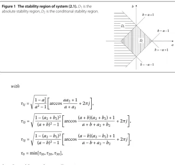
Figure 1 The stability region of system (2.1).D1is the
absolute stability region,D2is the conditional stability region.
with
τj=
–a a–
arccosaa+ a+a
+ πj
,
τj=
– (a+b) (a+b)–
arccos(a+b)(a+b) + a+b+a+b
+ πj
,
τj=
– (a–b) (a–b)–
arccos(a–b)(a–b) + a–b+a–b
+ πj
,
τ=min[τ,τ,τ],
where Dand Dare shown in Figure.
Proof From hypotheses (H) and (H), the characteristic equation associated with the lin-earization of system (.) is
(λ)(λ)(λ) = ,
where
(λ) =λ+ – (a+aλ)e–λτ,
(λ) =λ+ –
a+b+ (a+b)λ
e–λτ,
(λ) =λ+ –
a–b+ (a–b)λ
e–λτ.
Separately analyzing the roots ofi(λ) = (i= , , ), by using the method in [], we
have the following results.
If –≤a< , then all roots of(λ) = have negative real parts for allτ≥. Ifa< –, then(λ) = has a pair of purely imaginary roots whenτ=τj.
If –≤a+b< , then all roots of(λ) = have negative real parts for allτ ≥. If
a+b< –, then(λ) = has a pair of purely imaginary roots whenτ =τj.
If –≤a–b< , then all roots of(λ) = have negative real parts for allτ ≥. If
a–b< –, then(λ) = has a pair of purely imaginary roots whenτ=τj.
Summarizing the conclusions above, the proof is completed.
3 Properties of Hopf bifurcation
In the previous section, we have obtained the sufficient conditions for system (.) to un-dergo a Hopf bifurcation at the origin withτas a bifurcation parameter. In this section, we shall investigate the direction of the Hopf bifurcation and stability of bifurcating periodic solutions by takingf(u) =g(u) =u. Rewrite Eq. (.) as the following system:
The characteristic equation associated with the linearization of system (.) around the origin is given by
(γE–Aτ)eγ–Cγ – (B+B)τ = . (.)
Comparing with the previous characteristic equation, we findγ =λτ. For convenience, we denote γ = (τj+ν)λ, whereτj=τsj (s= , , ;j= , , , . . .) andν∈R. According to
Theorem , we know that system (.) undergoes a Hopf bifurcation at the origin when ν= .
By the Riesz representation theorem, there exist functionsη(θ) andμ(θ) such that
D(τ,φ) =φ() –
In fact, we can choose
Define
A(τ)φ=
dφ(θ)
dθ , θ∈[–, ),
φ(θ) –Cφ(θ) +Lφ, θ=
and
R(τ)φ=
, θ∈[–, ),
F(ν,φ), θ= .
Then Eq. (.) can be written as the abstract ODE,i.e.,
˙
Yt=A(τ)Yt+R(τ)Yt. (.)
The adjoint operatorA∗is defined byA∗= –ddsψ with the domain
DA∗=
ψ∈C∗=C[,τ],R:Ddψ
ds ∈C
∗;Ddψ
ds = –Lψ
.
We define the bilinear form:
ψ,φ =ψ¯()φ() –
–
d
θ
a= ¯
ψ(θ–a)dμ(a)
φ(θ)
–
–
s
θ= ¯
ψ(θ–s)dη(a)φ(θ)dθ.
It is not difficult to verify thatq(θ) =qeiωτjθ(θ∈[–, ]) andq∗(s) =lq∗ei
ωτjs(s∈[, ])
are the eigenvectors ofA() andA∗ corresponding to the eigenvaluesiωτjand –iωτj,
respectively, where
l=q∗I–Ce–iωτj+ (B
+B)τje–iωτj
¯
q
– ,
andq∗,q = . Now we compute the center manifoldCatν= . Define
z(t) =q∗,yt, W(t,θ) =yt(θ) – Rez(t)q(θ),
then we have
˙
z(t) =iωτjz+q¯∗()F(,yt). (.)
Equation (.) can be written in the abbreviated form
˙
z(t) =iωτjz+g(z,¯z), (.)
with
g(z,¯z) =g
z
+gz¯z+g ¯
z
+g
zz¯
Noting thatyt(θ) =W(t,θ) +z(t)q(θ) +z¯(t)q¯(θ), we have and comparing its coefficients with that of Eq. (.) gives that
g=g=g=
It is well known that the coefficientc() of third degree term of Poincaré normal form of Eq. (.) is given by []
Consequently, we have the following theorem on the bifurcating periodic solution.
Theorem For system(.),assume <a<
bifurcating periodic solutions are asymptotically stable;
() iff() < ,the direction of the Hopf bifurcation atτ=τjis subcritical and the
bifurcating periodic solutions are unstable.
Proof Whenτ=τj, by calculation, we easily obtain the following results:
If <a< √
,a< –
a andf
() > (< ), thenRec
() < (> ). Therefore, fromα(τj) >
, we have
μ= –
Re{c()} α(τj)
> (< ), β= Re
c()< (> ).
This completes the proof of Theorem .
Similarly, we can prove Theorem and Theorem , we omit the proof here.
Theorem For system(.),assume <a+b< √
,a+b< –
a+b,then
() ifaf() +bg() > ,the direction of the Hopf bifurcation atτ=τjis subcritical
and the bifurcating periodic solutions are unstable;
() ifaf() +bg() < ,the direction of the Hopf bifurcation atτ=τjis supercritical
and the bifurcating periodic solutions are asymptotically stable.
Theorem For system(.),assume <a–b< √
,a–b< –
a–b,then
() ifaf() –bg() > ,the direction of the Hopf bifurcation atτ =τjis subcritical
and the bifurcating periodic solutions are unstable;
() ifaf() –bg() < ,the direction of the Hopf bifurcation atτ =τjis supercritical
and the bifurcating periodic solutions are asymptotically stable.
4 Permanent oscillation
Based on Chafee’s criterion, if system (.) has a unique equilibrium point which is unsta-ble, and the solutions of system (.) are globally bounded, this system generates a limit cycle, namely a permanent oscillation [].
We consider system (.) and assume thatf,g,f,g are nonlinear bounded functions and satisfy Lipschitz condition,
|f(x) –f(y)| |x–y| ≤L,
|g(x) –g(y)| |x–y| ≤L.
We have the following lemmas.
Lemma If|α|L+|β|L< holds,system(.)has a unique equilibrium point.
Proof Suppose thatX∗is the equilibrium point of the system, then we have
AX∗+Bf
X∗+Bg
X∗= .
We define a mappingH:R→R
H(X) =AX+Bf(X) +Bg(X)
and assumeH(u) =H(v), then
(u–v) =
⎛ ⎜ ⎝
– +ac db db – +ac db db – +ac
⎞ ⎟
where|ci| ≤L,|dj| ≤L(i= , , ;j= , ). Under the given condition,is an invertible matrix. Thenu=v, namelyH(X) is injective onR. Noting thatf andgare bounded con-tinuous functions, it is easily to obtain thatH(u) → ∞, whenu → ∞. SoH(X) is a homeomorphism onRand system (.) has a unique equilibrium point.
Lemma The solutions of system(.)are globally bounded.
Proof Sincef,g,fandgare bounded continuous functions, there isM> such that
d|xi(t)|
dt ≤–xi(t)+M,
withi= , , . This proves the lemma.
Lemma The equilibrium point(, , )of system(.)is unstable when one of the
follow-ing conditions are satisfied:
() α> ,α>ατ,andτ+ ( –αατ) <αe –(–αα
τ),
() α+β> ,α+β> (α+β)τ,andτ+ ( –αα++ββτ) < (α+β)e –(–αα+β
+βτ), () α–β> ,α–β> (α–β)τ,andτ+ ( –αα––ββτ) < (α–β)e
–(–αα–β –βτ).
Proof Based on analysis in [], we know the roots of the following equation:
λ+ – (α+αλ)e–λτ= (.)
are the characteristic roots of the linearized system of (.). When condition () holds, Eq. (.) has at least a positive real root, and the equilibrium point (, , ) of system (.) is unstable.
Using the same method, we can obtain conditions () and (). The proof of the lemma
is completed.
Up to now, we have prepared sufficiently to state the following results.
Theorem System(.)generates a permanent oscillation,when|α|L+|β|L< holds
and one of the following conditions are satisfied: () α> ,α>ατ,andτ+ ( – α
ατ) <αe –(–αατ),
() α+β> ,α+β> (α+β)τ,andτ+ ( –αα++ββτ) < (α+β)e –(–αα+β
+βτ), () α–β> ,α–β> (α–β)τ,andτ+ ( –αα–β
–βτ) < (α–β)e –(–αα–β
–βτ).
5 Numerical simulation
In the section, we carry out some numerical simulations for system (.).
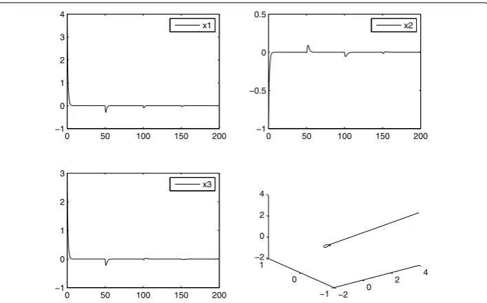
Assume thatα= .,β= .,α= . andβ= .. From Theorem , the zero solution of system (.) is absolutely stable. The simulation results as shown in Figure .
Figure 2 For system (2.1), whenτ= 50, the zero solution is asymptotically stable.
Figure 3 For system (2.1), whenτ= 0.47 <τ20= 0.48, the zero solution is asymptotically stable.
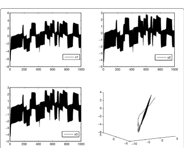
unstable, and system (.) undergoes a Hopf bifurcation at the origin whenτ=τ. Fur-thermore, the direction of the Hopf bifurcation atτ=τjis subcritical and the bifurcating
periodic solutions are unstable. The simulation results as shown in Figures and . Consider system (.) withα= .,β= .,α= andβ= , then we can chooseτ= , satisfying Theorem . System (.) generates a permanent oscillation (see Figure ).
6 Conclusion
Figure 4 For system (2.1), the bifurcating periodic solution is unstable whenτ= 0.54 >τ20= 0.48.
As we know, the extension of local periodic solutions for large time delay would appear when some conditions are satisfied. Further study of the patterns is undergoing.
Competing interests
The authors declare that they have no competing interests.
Authors’ contributions
The authors have achieved equal contributions to each part of this paper. All the authors read and approved the final manuscript.
Acknowledgements
The authors are very grateful to the referees for their valuable suggestions. This work is supported by the Fundamental Research Funds for the Central Universities (No. DL12BB29) and the National Natural Science Foundation of China (Grant No. 41304093).
Received: 31 January 2013 Accepted: 28 October 2013 Published:22 Nov 2013
References
1. Li, L, Yuan, Y: Dynamics in three cells with multiple time delays. Nonlinear Anal., Real World Appl.9, 725-746 (2008) 2. Luo, S, Liu, M, Xu, X: Stability analysis of class of neutral three neurons network with delay. J. Nat. Sci. Heilongjiang Univ.
3, 336-340 (2010)
3. Wei, J, Ruan, S: Stability and global Hopf bifurcation for neutral differential equations. Acta Math. Sin.45, 94-104 (2002) 4. Hassard, B, Kazarinoff, N, Wan, Y: Theory and Applications of Hopf Bifurcation. Cambridge University Press, Cambridge
(1981)
5. Chafee, N: A bifurcation problem for a functional differential equation of finitely retarded type. J. Math. Anal. Appl.35, 312-348 (1971)
10.1186/1687-1847-2013-338