Ionospheric multiple stratifications and irregularities induced by the 2011 off the Pacific coast of Tohoku Earthquake

(1)

Ionospheric multiple stratiﬁcations and irregularities induced by

the 2011 off the Paciﬁc coast of Tohoku Earthquake

Takashi Maruyama1_{, Takuya Tsugawa}1_{, Hisao Kato}1_{, Akinori Saito}2_{, Yuichi Otsuka}3_{, and Michi Nishioka}3

1_{National Institute of Information and Communications Technology, 2-1 Nukuikita 4-chome, Koganei, Tokyo 184-8795, Japan} 2_{Department of Geophysics, Graduate School of Science, Kyoto University, Kitashirakawa-Oiwake-cho, Sakyo-ku, Kyoto 606-8502, Japan}

3_{Solar-Terrestrial Environment Laboratory, Nagoya University, Furo-cho, Chikusa-ku, Nagoya 464-8601, Japan}

(Received April 8, 2011; Revised May 19, 2011; Accepted June 7, 2011; Online published September 27, 2011)

A strong earthquake with a magnitude of 9.0 occurred at 1446:23 JST on March 11, 2011, in Japan. Ionospheric disturbances were detected at 1500 JST at four ionosonde stations. An irregular distortion of echo trace was observed at Kokubunji, which is the nearest station to the epicenter and is 440 km from it. Multiple-cusp-type trace indicating extra stratiﬁcation was observed at Wakkanai and Yamagawa, which are 870 and 1410 km away from the epicenter. A small wavy ﬂuctuation was observed at Okinawa 1910 km away from the epicenter. The real height analysis of the ionograms showed a vertical structure with a scale size of 20∼30 km.

Key words:Ionospheric disturbance, earthquake,F1cusp enhancement, intermediate layer, stratiﬁcation.

1. Introduction

Perturbation of the ionosphere can occur after earth-quakes by way of dynamic coupling between seismic waves and the atmosphere (e.g., Shinagawaet al., 2007). Distur-bances in the ionospheric total electron content (TEC) are often reported associated with strong earthquakes (Heki and Ping, 2005; Hekiet al., 2006; Liuet al., 2006; Otsukaet al., 2006).

TEC measurement using radio signals transmitted from GPS satellites has a large advantage of high time and spatial resolutions. However, it is not very easy to detect any verti-cal structure because TEC values are an integrated quantity along the radio propagation path penetrating the ionosphere. On the other hand, ionosondes are limited in their number and location and usually they are programmed to run at in-tervals of several tenths of minutes. Despite such disadvan-tages their high capability in measuring vertical structure is expected to compensate TEC measurements. However, ob-servations of earthquake-induced ionospheric deformation in ionograms are quite rare and almost nothing has been re-ported except in the case of theM9.2 Alaska earthquake in 1964 (Leonard and Barnes, 1965).

A strong earthquake with a magnitude of 9.0 occurred off the Paciﬁc coast of Tohoku at 1446:23 JST (UT+9 hr) on March 11, 2011. Associated with the earthquake, striking ionospheric disturbance was observed. This paper describes ionospheric disturbances in ionograms obtained at four lo-cations over Japan.

Copyright cThe Society of Geomagnetism and Earth, Planetary and Space Sci-ences (SGEPSS); The Seismological Society of Japan; The Volcanological Society of Japan; The Geodetic Society of Japan; The Japanese Society for Planetary Sci-ences; TERRAPUB.

doi:10.5047/eps.2011.06.008

2. Ionospheric Measurements

Figure 1 shows aTEC map, showing the deviation of TEC from a smoothed background, (Tsugawaet al., 2011) as measured by the GPS receiver network, GEONET, in the center, and ionograms for the four stations at around 1445 JST (0545 UT) just prior to the earthquake. The oper-ation of the four ionosondes are programmed with a small time shift from the nominal time stamp of each quarter hour by−105,−30,+45, and+120 s for Wakkanai (45.16◦N, 141.75◦E), Kokubunji (35.71◦N, 139.49◦E), Yamagawa (31.2◦N, 130.62◦E), and Okinawa (26.68◦N, 128.15◦E), re-spectively. The sweep rate of the ionosondes is 2 MHz/s. In the three ionograms except for Wakkanai, sporadicEtraces separated into O- and X-modes were observed and these traces are not a signature of disturbance. A large retarda-tion of the trace near 3 MHz at Wakkanai corresponds to the

E-layer critical frequency (fOE), and a kink near 5 MHz at

Yamagawa is theF1cusp; both the signatures are also

nor-mal.

2.1 Perspective of the disturbance

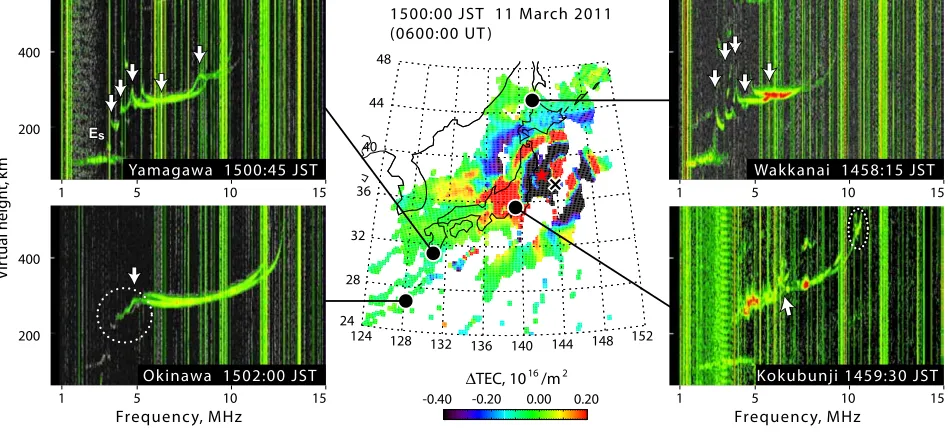
Figure 2 shows data in the same format as Fig. 1, ap-proximately 14 min after the earthquake. Striking TEC disturbance forming a concentric ring pattern and patchy disturbance are observed near 36◦N. The center of the concentric ring is shifted from the epicenter as shown by the red star (Tsugawaet al., 2011). Because we are dis-cussing ionospheric signatures, the center of the ring pat-tern is considered to be a source of the atmospheric dis-turbance and is referred to as the ionospheric epicenter, which is shown by the cross in theTEC map. Distances of the ionosonde location from the ionospheric epicenter are 440 km (Kokubunji), 870 km (Wakkanai), 1410 km (Yamagawa), and 1910 km (Okinawa), the corresponding ionograms are shown counterclockwise from the bottom right. Detailed analysis of the ionogram at each location is presented as follows in the order of distance from the

(2)

Fig. 1. Ionospheric signature prior to the earthquake. The map in the center shows the TEC disturbance (Tsugawaet al., 2011) and the four ionograms are for Kokubunji (bottom right), Wakkanai (top right), Yamagawa (top left), and Okinawa (bottom left) in the order of distance from the epicenter.

Fig. 2. The same as Fig. 1 but approximately 14 min after the earthquake. Note that the ionogram times delayed with lowering the latitude and the observation at Okinawa was 2 min after theTEC map. The arrows indicate a cusp signature for the O-mode trace. The red star in the TEC map is the epicenter reported by the U.S. Geological Survey, while the cross shows the center of the concentric circle of TEC disturbance (ionospheric epicenter).

centers.

Kokubunji

The whole F trace showed irregular distortion with a kink near 6.5 MHz as shown by the arrow, above which the trace was split showing a non-vertical reﬂection (the oblique trace was not fully connected). The frequency of the kink is much higher than theF1cusp normally observed

(∼4.5 MHz) as shown by the arrow in Fig. 1. Near the critical frequency of the X-mode wave at 10.5 MHz, the trace was distorted as circled by the dotted line, which indicates that the disturbance reached theF2peak height at

306 km determined from the transmission factor,M3000F2.

TheF2peak height was raised by 27 km as compared with

the previous ionogram for 1444:30 JST.

Wakkanai

Signiﬁcant disturbance was observed with much more or-ganized traces as compared with Kokubunji. The retarda-tion of the lowest part of theFtrace corresponds to fOEas

in the case of the ionogram for 1443:15 JST, except for the height which was lowered by approximately 20 km. The trace was disrupted at 3.4 MHz showing the appearance of a new layer above. The next layer showed an enhanced cusp at 3.96 MHz, which is close to the frequency of the normalF1cusp (4∼4.2 MHz) as indicated by ionograms at

the same local time on other days. Two more weak cusps were noted at around 4.6 and 5.9 MHz in theF2region. The

(3)

Fig. 3. (a) Sketch of ionogram O-mode trace (solid line) and synthesized X-mode trace (dotted line) from the real height density profile; (b) real height density profile (red line) converted from the scaled O-mode trace shown in panel (a) using POLAN. The blue thin line is the density pro-file for 1445:45 JST for reference. The electron density is represented by the corresponding plasma frequency (f[Hz]=8.98√ne, wherene

is the electron density in [m−3_{]) to relate the ionogram and the density}

proﬁle.

at 105 (E-layer peak), 130, 153, 173, and 199 km. The ex-trapolatedF2peak was at 255 km. (For more details of this

analysis, see below for Yamagawa.)

Yamagawa

The disturbance signature was very similar to that of Wakkanai (the O-X mode identiﬁcation by eye is easier than Wakkanai except in a 6–7.5 MHz range). A weak sporadic

E layer blanketed the lowest part of the upper trace in a frequency range 3.44–3.68 MHz. A discontinuity can be noted at 4.15 MHz and two well-deﬁned cusps were at 4.75 and 8.40 MHz. The ﬁrst of the two cusps was close to the F1cusp at∼4.6 MHz as noted (fOF1) in the ionogram

for 1445:45 JST. A careful examination with an assist of POLAN showed another cusp at 6.30 MHz.

Figure 3(a) is a sketch of the ionogram showing the scaled O-mode trace (solid line) and the synthesized X-mode trace (dotted line) from the real height density pro-ﬁle. The real height proﬁle was obtained from the O-mode trace by POLAN and O-mode scaling was adjusted until self-consistent O- and X-mode traces were obtained.

Thus, overlapping traces were resolved in the 6–7.5 MHz range.

Figure 3(b) shows the real height density proﬁles. The red line corresponds to the ionogram in Fig. 3(a) and the blue thin line is obtained from the previous ionogram for 1445:45 JST.

Comparing the two diagrams, we see that small changes in the vertical density gradient yield large changes in the

vir-tual height of ionogram traces, and the characteristic heights were easily determined by combining the two. (The same analysis was conducted for Wakkanai and Okinawa.)

The height of the discontinuities were at 108 (E-layer peak), 133, 160, 191, and 224 km. The extrapolated F2

peak was at 262 km.

Okinawa

The disturbance was weak at Okinawa and the distortion showed a wavy pattern as circled by the dotted line in the bottom left panel of Fig. 2. The heights of the discontinuity were at 111 (E-layer peak), 141, 158, and 175 km. The last cusp was considered to be the normalF1cusp as determined

from the ionogram at the same local time on the previous day; theF1cusp was moderately enhanced when compared

with the previous frame of the ionogram in Fig. 1.

Thus the disturbance was limited in theF1region, unlike

in the case of the other stations.

The extrapolatedF2peak was at 298 km.

2.2 Commencement of the disturbance

The ionosondes are routinely operated at 15-min inter-vals. In addition to this, experimental mode soundings are scheduled at 5 min to each hour at Wakkanai. No distur-bance was observed in this extra ionogram for 1455:00 JST at Wakkanai, and the disturbance commenced at 1458:15 JST there. Considering the distance of 870 km from the ionospheric epicenter, the apparent propagation velocity of the perturbation was estimated to be faster than 1220 m/s but slower than 1670 m/s. If the same velocity is applied to the South-West direction, the disturbance is expected to appear on the ionogram at a time between 1500:30 and 1505:30 JST at Yamagawa, and the actual observation was in the frame of 1500:45 JST as shown in Fig. 2.

Therefore, the times of commencement at Wakkanai and Yamagawa were consistent and the apparent propagation velocity was estimated to be at the faster end of the am-biguity range between 1220 and 1670 m/s.

At Okinawa, however, the expected time is between 1505:30 and 1512:30 JST and the actual observation was in the frame of 1502:00 JST. The disturbance was observed 3.5 min earlier than the expected time and the apparent ve-locity was estimated to be 2038 m/s.

Liu and Sun (2011) determined velocities of seismo-traveling ionospheric disturbances induced by the same earthquake for several modes. The velocities are 2100– 3200, 900, and 200 m/s for Rayleigh waves, acoustic grav-ity waves, and tsunami waves, respectively. The com-mencement of the ionogram signatures of disturbance was close to the range of propagation time of the Rayleigh wave, which might excite atmospheric waves having a slower propagation velocity.

2.3 Time evolution

(4)

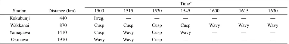
Table 1. Summary of disturbance signatures.

Time∗

Station Distance (km) 1500 1515 1530 1545 1600 1615 1630

Kokubunji 440 Irreg. — — — — — —

Wakkanai 870 Cusp Cusp Cusp Cusp Wavy Wavy Wavy

Yamagawa 1410 Cusp Wavy Cusp Wavy — — —

Okinawa 1910 Wavy Wavy Cusp — — — —

∗_{The actual observation times are shifted depending on the station, see the text for details.}

“Irreg.”, “Cusp”, and “Wavy” stand for irregular distortion of the trace, steep cusp signature, and consecutive weak cusp signature in the ionogram.

once showed a weak wavy pattern at 1515 JST, and mul-tiple enhanced cusps reappeared in the F1 andF2 regions

at 1530 JST. After this, the trace returned to a wavy pat-tern at 1545 JST. At 1600 JST, the disturbance disappeared in the frequency range higher than 4.36 MHz, below which sporadicE layer blanketed theF trace. The disturbance at Okinawa was a wavy pattern at 1500 and 1515 JST. The

F1cusp was enhanced and a weak cusp appeared in theF2

region at 1530 JST. The disturbance almost disappeared at 1545 JST.

The time evolution at the four locations is summarized in Table 1.

2.4 Vertical scale of the disturbance

At Kokubunji, the disturbance extended from the sup-posedF1 cusp (∼4.7 MHz) up to theF2peak 13 min after

the quake, though the F1 trace was blanketed by the

spo-radicElayer. The disturbance was signiﬁcant at lower alti-tudes.

Ionogram signatures at Wakkanai and Yamagawa at 1500 JST were quite similar to each other such that:

(1) The lowest part of the distortion was between theE -layer peak and the F1 cusp. The ionogram trace

re-sembled an intermediate layer or high-type sporadicE

layer showing an abrupt transition to the upper layer. (2) A steep cusp was near theF1-layer critical frequency

(fOF1). The fOF1is mostly determined by a chemical

process and shows a small day-to-day variability, un-like fOF2. Therefore, the enhancement of theF1cusp

may not be a purely dynamical one but there seems to be contribution of a chemical process including re-combination.

(3) Two cusps were in theF2region; a barely-deﬁned one

at lower altitude and a moderate one at higher alti-tude. The vertical separation of the two cusps was 26 and 33 km at Wakkanai and Yamagawa, respectively. The separation between the enhancedF1cusp and the

barely-deﬁned lower cusp in theF2region was 20 and

31 km at Wakkanai and Yamagawa, respectively. Although the disturbance at Okinawa was weaker as compared with the other stations, several common features with Wakkanai and Yamagawa were observed. The low-est part of the distortion of the ionogram, a faint segment between 3.6 and 3.9 MHz inside the circle, was the inter-mediate layer. Comparing the ionograms at 1447:00 and 1502:00 JST, we note that the F1 cusp was evidently

en-hanced.

2.5 Peculiarity of Kokubunji ionogram

The ionospheric disturbance at Kokubunji was different in many aspects from the other three stations. The ionogram traces showed irregular distortion only at Kokubunji. The

F-layer peak was raised by 27 km in 15 min at Kokubunji, while it remained at the same level at the other stations. The enhancement of theF1cusp was not seen at Kokubunji. The TEC map in Fig. 2 shows that there coexisted two types of TEC perturbations; a patchy pattern of TEC enhancement was noted at Kokubunji, which can be distinguished from the concentric pattern. The patchy pattern moved fast out of this area (Tsugawaet al., 2011). The unique signature of the ionogram distortion and its short duration time at Kokubunji might be related to this type of TEC disturbance.

3. Summary

The 2011 off the Pacific coast of Tohoku Earthquake oc-curred at 1446:23 JST (0546:23 UT) on March 11, 2011. Associated with the earthquake, ionospheric disturbance was detected approximately 14 min after the earthquake in quarter-hourly ionograms obtained at four locations from north to south along the Japanese archipelago. The distur-bance was characterized by a vertical structure that is diffi-cult to detect by TEC measurement using trans-ionospheric radio waves. Multiple stratifications were observed at Wakkanai, Yamagawa, and Okinawa such that an appear-ance of an intermediate layer or high-type sporadicElayer, an enhancement of theF1cusp, and additional cusps in the

F2region. The vertical scale of the distortion,

correspond-ing to the separation of the two consecutive cusps, was the order of 20∼30 km.

The disturbance at Kokubunji, the closest station to the epicenter, was different in many aspects from the other sta-tions. The ionogram trace showed irregular distortion and theF-layer peak was raised by 27 km after the earthquake. The enhancedF1 cusp and the intermediate layer were not

observed.

Acknowledgments. The GPS data are provided by the Geospatial Information Authority of Japan. The authors thank J. Uemoto for running POLAN.

References

Heki, K. and J. S. Ping, Directivity and apparent velocity of the coseis-mic ionospheric disturbances observed with a dense GPS array,Earth Planet. Sci. Lett.,236, 845–855, 2005.

(5)

Leonard, R. S. and R. A. Barnes, Observation of ionospheric disturbances following the Alaska earthquake,J. Geophys. Res., 70, 1250–1253, 1965.

Liu, J.-Y. and Y.-Y. Sun, Seismo-traveling ionospheric disturbances of ionograms observed during the 2011Mw9.0 Tohoku Earthquake,Earth

Planets Space,63, this issue, 897–902, 2011.

Liu, J.-Y., Y.-B. Tsai, K.-F. Ma, Y.-I. Chen, H.-F. Tsai, C.-H. Lin, M. Kamogawa, and C.-P. Lee, Ionospheric GPS total electron content (TEC) disturbances triggered by the 26 December 2004 Indian Ocean tsunami,J. Geophys. Res.,111, A05303, doi:10.1029/2005JA011200, 2006.

Otsuka, Y., N. Kotake, T. Tsugawa, K. Shiokawa, T. Ogawa, Effendy, S. Saito, M. Kawamura, T. Maruyama, N. Hemmakorn, and T. Komolmis, GPS detection of total electron content variations over Indonesia and Thailand following the 26 December 2004 earthquake,Earth Planets Space,58, 159–165, 2006.

Shinagawa, H., T. Iyemori, S. Saito, and T. Maruyama, A numerical sim-ulation of ionospheric and atmospheric variations associated with the Sumatra earthquake on December 26, 2004,Earth Planets Space,59, 1015–1026, 2007.

Titheridge, J. E., The real height analysis of ionograms: A generalized formulation,Radio Sci.,23, 831–849, 1988.

Tsugawa, T., A. Saito, Y. Otsuka, M. Nishioka, T. Maruyama, H. Kato, T. Nagatsuma, and K. T. Murata, Ionospheric disturbances detected by GPS total electron content observation after the 2011 off the Paciﬁc coast of Tohoku Earthquake,Earth Planets Space,63, this issue, 875– 879, 2011.