A general neuro space mapping technique for microwave device modeling

R E S E A R C H

Open Access

A general neuro-space mapping technique

for microwave device modeling

Lin Zhu

, Jian Zhao

, Zhuo Li

, Wenyuan Liu

, Lei Pan

, Haifeng Wu

and Deliang Liu

Abstract

Accurate modeling of nonlinear microwave devices is critical for reliable design of microwave circuit and system. In this paper, a more general neuro-space mapping (Neuro-SM) method is proposed to fulfill the needs of the increased modeling complexity. The proposed technique retains the capability of the existing dynamic Neuro-SM in modifying the dynamic voltage relationship between the coarse model and the desired model. The proposed Neuro-SM also considers dynamic current mapping besides voltage mappings. In this way, the proposed Neuro-SM generalizes the previously published Neuro-SM methods and has the potential to produce a more accurate model of microwave devices with more dynamics and nonlinearity. A new formulation and new sensitivity analysis technique are derived to train the general Neuro-SM with dc, small-, and large-signal data. A new gradient-based training algorithm is also proposed to speed up the training. The validity and efficiency of the general Neuro-SM method are demonstrated through a real 2 × 50 μm GaAs pseudomorphic high-electron mobility transistor (pHEMT) modeling example. The proposed general Neuro-SM model can be implemented into circuit simulators conveniently.

Keywords: Artificial neural network, Space mapping, Neuro-SM, Microwave device modeling

1 Introduction

Microwave transistors are key components in the next

generation wireless communication systems [1–4],

such as cognitive multiple-input multiple-output

(MIMO) systems [5–7], and cognitive relay network

[8, 9]. With the increasing complexity of

communica-tion circuit and system structure, designers rely more heavily on computer-aided design (CAD) software to achieve efficient design. Microwave device models are essential to CAD software. The accuracy of these models can even decide whether the communication circuit and system design is successful or not. Due to rapid technology development in semiconductor in-dustry, new microwave devices constantly arrive. Models suitable for previous devices may not fit new devices well. There is an ongoing need for new accur-ate models.

In recent years, neuro-space mapping (Neuro-SM)

technique [10] combining artificial neural networks

[11] with space mapping [12] has been recognized in

microwave device modeling with the advantages of good efficiency and accuracy. In Neuro-SM, neural networks are used to automatically map and modify an existing equivalent circuit model also called coarse model to a desired/accurate model through a process named training. In order to fulfill the needs of the

increased modeling complexity and the industry’s

in-creasing need for tighter accuracy, several

improve-ments on the basis of [10] were subsequently studied

to enhance the modeling accuracy and efficiency,

such as Neuro-SM with the output mapping [13],

dy-namic Neuro-SM [14], and analytical Neuro-SM with

sensitivity analysis [15]. Neuro-SM with the output

mapping [13] was introduced, through incorporation

of a new output/current mapping, for modeling of microwave devices. Compared to the Neuro-SM

* Correspondence:[email protected]

1_{School of Control and Mechanical Engineering, Tianjin Chengjian University,} Tianjin 300384, China

Full list of author information is available at the end of the article

presented in [10], Neuro-SM with the output map-ping is more suitable for modeling nonlinear devices with more nonlinearity due to the additional and useful degrees of freedom from the output mapping neural network. In order to accurately model nonlin-ear devices which have higher order dynamic effects (e.g., capacitive effect or non-quasi-static effect) than that of the coarse model, dynamic Neuro-SM was

in-troduced [14]. However, when the modeling devices

have both more nonlinearity and high order dynam-ics, in such case, even though existing Neuro-SM

[13, 14] is used to map the coarse model towards

the device data, the match between the trained Neuro-SM models and the device data may be still not good enough. More effective Neuro-SM methods need to be investigated to overcome the accuracy limit of the Neuro-SM presented in [13, 14].

In this paper, we propose a more generalized Neuro-SM approach including not only static map-ping but also dynamic mapmap-ping, and considering both voltage mapping and current mapping for the first time. This paper is a further expansion of the work in [13, 14]. Compared to [13] where only static mapping is used, the proposed technique is more suitable for modeling nonlinear devices with higher order dynamic effects and non-quasi-static effect that may be missing in the coarse model due to

in-clusion of dynamic mapping. Compared to [14], the

general Neuro-SM considers not only input voltage mapping, but also output current mapping, further refining the existing coarse model. In this way, well trained general Neuro-SM model can represent the dynamic behavior and large-signal nonlinearity of the microwave devices more accurately than the coarse model, Neuro-SM model with the output mapping

[13], as well as dynamic Neuro-SM model [14]. The

modeling results of a real 2 × 50 μm GaAs

pseudo-morphic high-electron mobility transistor (pHEMT) demonstrate the correctness and validity of the pro-posed general Neuro-SM technique.

2 Concept of the general Neuro-SM model

Suppose the existing equivalent circuit model is a rough approximation of the behavior of the micro-wave device. We name this existing model as the coarse model. Let the desired model that accurately matches the device data be called the fine model. Just take field effect transistor (FET) modeling as an example, let the gate and drain voltages and currents of the coarse model be defined as vc= [vc1,vc2]T and ic= [ic1,ic2]T, respectively. Let the terminal voltages

and currents of the fine model as vf= [vf1,vf2]T and if= [if1,if2]T, respectively.

Suppose the total number of voltage delay buffers

at gate and drain be the same and both equal to Nv.

Let τ be the time delay parameter. To represent

time-domain behavior, the time parameter t is

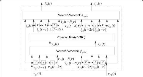
intro-duced. Figure 1 illustrates the signal flow of the

general Neuro-SM model. At first, the present volt-ages of the fine model vf(t) as well as their

histor-yvf(t−τ), vf(t−2τ), …, and vf(t−Nvτ) are mapped

into the coarse model voltages vc(t). Because the

formula of the mapping is unknown and usually nonlinear, a neural network is used to learn and represent the mapping. While the Neuro-SM

pre-sented in [10] uses a static neural network such as

multilayer perceptron (MLP), we propose to use a time delay neural network (TDNN) to map the coarse model to fine model. In functional form, vc(t)

can be described as

vcð Þ ¼t fANN vfð Þt ;vfðt−τÞ;…;vfðt−NvτÞ;w1

;Nv≥0

ð1Þ

where fANN represents the input/voltage mapping

neural network, and w1 is a vector containing all the

weights of the input mapping neural network. As

seen from Eq. (1), voltages at gate and drain of the

coarse model depend on not only the present voltages of the fine model, but also their history sig-nals making the proposed technique more suitable for modeling the dynamic behavior of the nonlinear devices. Then, after the coarse model computation,

the coarse model currents ic(t) can be obtained.

Sup-pose the total number of current delay buffers at

gate and drain be the same and both equal to Nc. At

last, ic(t) and their history ic(t−τ), …, ic(t−Ncτ) as

well as the present voltages of the fine model vf(t)

are mapped by another TDNN to the external cur-rents as

ifð Þ ¼t hANN vfð Þt ;icð Þt ;icðt−τÞ;…;icðt−NcτÞ;w2

;Nc≥0

ð2Þ

where hANN represents the output/current neural

network, and vector w2 contains all the output

map-ping neural network weights. Compared to [14], the

new output neural network mapping further refines the coarse model current signals to produce the fine model outputs. The combined dynamic voltage map-ping neural network, coarse model, and dynamic current mapping neural network is called the general Neuro-SM model.

The proposed general Neuro-SM is more general

than Neuro-SM technique presented in [10, 13, 14].

While N_v= 0, then the general Neuro-SM model

without the output mapping is static Neuro-SM

model [10]. While Nv= 0 and Nc= 0, then the

gen-eral Neuro-SM model belongs to the Neuro-SM

model with the output mapping [13]. While Nv > 0,

then the general Neuro-SM model without the

out-put mapping is the dynamic Neuro-SM model [14].

In this way, the proposed general Neuro-SM gener-alizes the previously published Neuro-SM technique. Furthermore, while Nv> 0 and Nc> 0, a new

Neuro-SM technique is presented for the first time.

Com-pared to the Neuro-SM introduced in [10, 13, 14],

the new Neuro-SM is more suitable for modeling the microwave devices with high order dynamics and nonlinearity due to inclusion of dynamic map-ping as well as current mapmap-ping.

3 Proposed analytical formulation of the general Neuro-SM model for training

The general Neuro-SM model will not be accurate unless the dynamic voltage and dynamic current mapping neural networks are trained suitable. In order to train the general Neuro-SM efficiently with

typical types of transistor modeling data, the

relationship between the dynamic voltage and

current mapping neural networks with typical types

of transistor data, such as DC, bias-dependent S

parameter, and large-signal harmonic data need to be derived.

In the DC case, present voltage signals of the fine model v_f(t) as well as its history, i.e.,v_f(t−τ), …, and vf(t−Nvτ) are all equal and defined as Vf, DC.

Simi-larly, present current signals of the coarse model i_c(t) as well as its history, i.e.,i_c(t−τ), …, and i_c(t−N_cτ)

are all equal and defined as I_c, DC. The response of

the general Neuro-SM model at V_f, DCcan be

gener-ally described as

The small-signal S parameter of the general

Neuro-SM model can be calculated by transforming its Y

parameters of the coarse model Yc. In functional form,Yf can be described as

YfðωÞ

¼ XNc

l¼0

e−jωlτ∂hTANNðvfðtÞ;icðtÞ;icðt−τÞ;…;icðt−NcτÞ;w2Þ

∂icðt−lτÞ

j

icðtÞ ¼icðt−τÞ ¼⋯¼icðt−NcτÞ ¼IcjVc;Bias

!

YcðωÞjVc;Bias

XNv

k¼0

e−jωkτ∂fANNT ðvfðtÞ;vfðt−τÞ;…;vfðt−NvτÞ;w1Þ

∂vfðt−kτÞ

j

vfðtÞ¼vfðt−τÞ¼⋯¼vfðt−NvτÞ¼Vf;Bias

!

þ ∂hTANNðvfðtÞ;icðtÞ;icðt−τÞ;…;icðt−NcτÞ;w2Þ

∂vfðtÞ

j

icðtÞ ¼icðt−τÞ ¼⋯¼icðt−NcτÞ ¼IcjVc;Bias

!

ð5Þ

where

Vc;Bias ¼fANNðVf;Bias;Vf;Bias;…;Vf;Bias;

z}|{Nvþ1

;w1Þ ð6Þ

where the first-order derivatives offANN andhANNcan be obtained at the biasVf, Biasusing adjoint neural network

method [15]. Superscriptkandl represent the index of voltage and current delay buffers, respectively. Equation (5)

includes two parts. The first part is in the form of multiplications of three matrices, which are defined as the output/

current Y-mapping matrix, i.e., the sum of products ofe−jωlτand ∂hANN/∂ic,Yparameter matrix of the coarse model

Yc, as well as the input/voltage Y-mapping matrix, i.e., the sum of products ofe−jωkτand∂fANN/∂vf. The other part is

the sensitivity matrix ofhANN. Equation (5) is more general than formulas of small-signalYparameter of the

Neuro-SM models in [10, 13, 14] due to the consideration of the new effects of current mappings and dynamic mappings.

For large-signal case, we need to derive the relationship between HB computation and dynamic voltage and current mapping neural networks so that model training can be performed with harmonic data. Let the harmonic current of

the general Neuro-SM model and coarse model at a generic harmonic frequencyωkbeIf(ωk) andIc(ωk), respectively.

TheIf(ωk) can be evaluated as

I

ð Þ¼

ω

N

1

X

n¼0

h

ðv

ð Þ

t

;

i

ð Þj

t

;

i

ð

t

−

τ

Þj

;

…

;

i

ð

t

−

N

τ

Þj

;

w

Þ

W

ð

n

;

k

Þ

ð7Þ

vcð Þ ¼tn fANN vfð Þtn ;vfðtn−τÞ;…;vfðtn−NvτÞ;w1

ð8Þ

vfðtn−mτÞ ¼ XNH

k¼0

Vfð Þ ωk e−jmωkτWNðn;kÞ;m¼0;1;…;Nv ð9Þ

where the subscript k represents the index of the harmonic frequency, k = 0, 1, 2, …, N_H, where N_H is the

number of harmonics considered in HB simulation. N_T is the number of time sampling points, W_N(n,k) is

the Fourier coefficient for the nth time sample and the k-th harmonic, superscript * denotes complex

conju-gate, and m represents the index of voltage delay buffers, m = 0, 1,…, N_v,. As seen from (7)~(9), apart from

changing the nonlinearity of the coarse model, dynamic voltage and current neural network mappings can also change the dynamic order so that the proposed general Neuro-SM has the potential to model the microwave devices with high order dynamics and nonlinearity.

4 Sensitivity analysis of the general Neuro-SM model with respect to mapping neural network weights

Let the number of hidden neurons of the dynamic voltage and current mapping neural networks be Nhv

and Nhc, respectively. Let generic symbols w1, i (i= 1, 2,…, Nhv) and w2, i (i= 1, 2,…,Nhc) be internal

weights of the voltage and current mapping neural network, respectively. w1, i and w2, i are the i-th

compo-nent of vectors w1 and w2, respectively. In order to train the general Neuro-SM efficiently, gradient

infor-mation provided by sensitivities of the model with respect to w1, i and w2, i is needed [16].

(1)DC sensitivity: let the DC output at gate and drain of the general Neuro-SM model beI_f, DC. The sensitivities of If, DCwith respect tow1,iandw2,iare described in functional form as

∂If;DC

∂w1;i ¼

∂IT f;DC

∂Ic;DC

!T

∂ITc;DC

∂Vc;DC

!T

∂Vc;DC

∂w1;i

¼ ∂hTANN

Vf;DC;Ic;DCVc;DC;Ic;DCVc;DC;…;Ic;DCVc;DC

z}|{Ncþ1

;w2

∂Ic;DC

!T

Gc

∂fANNðVf;DC;Vf;DC;…;Vf;DC zfflfflfflfflfflfflfflfflfflfflfflfflfflfflfflfflfflfflffl}|fflfflfflfflfflfflfflfflfflfflfflfflfflfflfflfflfflfflffl{Nvþ1

;w1Þ

∂w1;i

ð10Þ

∂If;DC

∂w2;i ¼

∂hANNðVf;DC;Ic;DCVc;DC;Ic;DCVc;DC;…;Ic;DCVc;DC

z}|{Ncþ1

;w2Þ

∂w2;i ð11Þ

where Gc¼ ð∂ITc;DC=∂Vc;DCÞ T

is the DC conductance matrix of the existing coarse model, and the first-order

derivatives ∂fANN/∂w1, i and ∂hANN/∂w2, i can be calculated by neural network backpropagation [17].

(2) S parameter sensitivity: S parameter sensitivity can be obtained by converting its Y parameter sensitivity.

The small-signal Y parameter sensitivities of the general Neuro-SM model with respect to w1, i and w2, i are

where the second-order derivative of the dynamic voltage and current mapping neural networks fANN and

hANN, which are the differentiation of the Jacobian matrix ∂fT_ANN=∂icðt−lτÞ and ∂fT_ANN=∂vfðt−kτÞ with respect

to w1, i and w2, i, can be obtained by the adjoint neural network back-propagation [17], respectively.

(3) HB sensitivity: the sensitivities of the large-signal harmonic current of the general Neuro-SM model with re-spect tow1,iandw2,iat a generic harmonic frequencyωk,k= 0, 1, 2,…,NHcan be described in functional form as

whereGc(tn) at the mapped voltage of coarse model vc(tn) is the nonlinear conductance matrix of the existing coarse

model at time pointtn.

5 Sensitivity analysis of the general Neuro-SM model with respect to coarse model parameters

Let x be a generic variable in the coarse model. In case the coarse model parameter needs to be treated as a

variable in circuit optimization, it is useful to obtain the sensitivity for DC, bias-dependentSparameter, and

large-signal HB responses of the general Neuro-SM model due to changes in the generic optimization variablex.

(1)DC sensitivity: the sensitivity ofI_f, DCwith respect toxis derived as

∂If;DC

(2)S parameter sensitivity:Sparameter sensitivity with respect to coarse model variablexcan also be calculated by converting itsYparameter sensitivity. TheYparameter sensitivity is shown as

where∂Yc/∂xis the sensitivity forYparameter of the coarse model due to changes inx.∂icr/∂x,r= 1, 2 is the

deriva-tive of coarse model current with respect tox,which can be calculated by coarse model sensitivity analysis.

(3) HB sensitivity: the sensitivity of the harmonic current of the general Neuro-SM model with respect tox at a generic harmonic frequencyωk,k= 0, 1,…,NH is shown in Eq. (18), where∂ic(tn)/∂xis the sensitivity of the

nonlin-ear current of the coarse model with respect toxat time sampletn.

∂Ifð Þωk

6 Proposed training algorithm for the general Neuro-SM model

Training is the key step to determine the general Neuro-SM model. The model development process needs two phases: initial training and formal training.

A.Initial training

Before the nonlinear device data from simulation or measurement is used for formal training, the general Neuro-SM model is first initialized to be equal to the original coarse model. In such case, the dynamic voltage and current neural networks are initialized to learn unit mappings, i.e., to learn the relationshipsv_c1(t) =vf1(t),vc2(t) =vf2(t),ic1(t)

=i_f1(t), andic2(t) =if2(t) in the entire operation range of the nonlinear device.

B.Formal training

In this phase, the weights of dynamic voltage and current mapping neural networks, i.e., w₁ and w₂, are

trained such that the overall training error of the general Neuro-SM model can be reduced to satisfy the

specifications. The overall training error for combined DC, small-signal S parameter, and large-signal HB

training is defined as the total difference between all nonlinear device data and the general Neuro-SM model as:

where I(.), S(.), and HB(.) are the DC, bias-dependent S parameter, and HB responses of the general Neuro-SM

model, respectively. Take FET modeling as an example, vector I(.) contains gate and drain current If1 and If2,

which can be computed by Eq. (3). Vector S(.) is achieved from the Y matrix defined by Eq. (5). HB responses

of the general Neuro-SM model, i.e., HB(.) can be calculated by Eq. (7). ID, SD, and HBD represent the DC

current, small-signal S parameter, and large-signal HB responses of the modeling device, respectively. The

sub-script k ðk¼1;2;…;NVf2Þ, l ðl¼1;2;…;NVf1Þ, j (j= 1, 2,…,Nfreq), m (m= 1, 2,…,NH), and n (n= 1, 2,…,NP)

denote the indices of Vf2,Vf1, frequency, harmonic frequency, and input power level, respectively. NVf1, NVf2,

Nfreq, NH, and NP are the total number of Vf1, Vf2,frequency, harmonic frequency, and input power level,

re-spectively. Diagonal matrices A, B, and C contain all the scaling factors, which are defined as the inverse of

the minimum-to-maximum range of the ID data, SD data, and HBD data, respectively. The training error

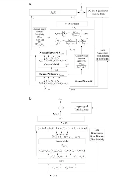
calcu-lation of the general Neuro-SM model for combined DC and S parameter training as well as HB training

fur-ther illustrates in Fig. 2. Figure 2a, b is error calculation for combined dc and small-signalS parameter training

The objective of the model training is to minimize the errorEdefined in (19) by optimizingw1and w2. In gen-eral, gradient-based training algorithm is used. After training, the general Neuro-SM model with appropriate hidden neurons and delay buffers can accurately repre-sent the nonlinear behavior of the modeling device.

7 Discussion

The proposed Neuro-SM model, after being trained for a specific range, is very good at representing the nonlin-ear behavior of the microwave device within the training region. However, when we use model in a wider range than the training range, inappropriate derivative infor-mation of the model outside the training range may mis-lead the iterative process into slow convergence or even divergence during large-signal simulation. One possible way to solve the divergence problem is to use

appropriate extrapolation technique. For general Neuro-SM technique, a simple and effective extrapolation technique is used to improve the convergence of the model [18].

For simplification, the proposed general Neuro-SM technique is formulated for 2-port field-effect transistor (FET) modeling. This approach can be further extended ton-port network, where all the notations and equations are extended accordingly. After the generalization, the proposed general Neuro-SM technique has the potential to be used for developing models of microwave devices with trapping effect.

The format of the general Neuro-SM model presented so far is to map the voltage input signals between the coarse and fine models. Hence, our approach presented so far is applicable to modeling voltage controlled devices, such as FET and HEMT. It is possible to extend

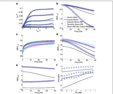
Fig. 3Comparison between the pHEMT device data, coarse model, and three Neuro-SM models.adc.b-eS parameter at two test biase points

the method to a mixed input mapping case, where the dynamic input mappings are for a mixture of port volt-age and current signals. In that way, our approach can be extended to modeling current controlled devices, such as HBT.

The frequency limit of the proposed general Neuro-SM model depends on the frequency limit of training data. For example, if the frequency in the training data extends to millimeter wave bands, the proposed general mapping will be even more important because of the need of capacitive effects, non-quasi-static effects, and

nonlinear effects in the model. In this case, more hidden neurons and time delay buffers maybe needed to guarantee the accuracy of the proposed general Neuro-SM model.

8 A pHEMT modeling using the proposed general Neuro-SM method

This example illustrates the use of the general

Neuro-SM for modeling of a real 2 × 50 μm GaAs pHEMT

device. The training and test data is obtained from measurement. An enhanced Angelov model including a

thermal subcircuit to model the self-heating effect of the device proposed in [19] is used as the existing coarse model. Even though parameters in enhanced Angelov model are extracted as much as possible, there are still distinct differences between the model and measured data. Thus, Neuro-SM is used to bridge the gap between the coarse model and measured data. We then apply the previously published Neuro-SM technique such as

Neuro-SM with the output mapping [13] and dynamic

Neuro-SM [14] to get more accurate models. After train-ing, the accuracy of the two Neuro-SM models is clearly improved compared to that of the coarse model, as

shown in Fig.3. However, the previous Neuro-SM

tech-niques at their best are still insufficient to achieve the desired accuracy. Then, our proposed general Neuro-SM is used to get a more accurate model.

Training was firstly done in NeuroModelerPlus

[20] using DC and bias-dependent S parameter data

for 400 iterations. Then, training refinement was

done using combined DC, bias-dependent S

param-eter, and HB data at 189 different biases for 3600 iterations. Harmonic data used for HB training was measured at 7.5 GHz fundamental frequency and

dif-ferent input power levels (−10~ 3 dBm). Time delay

parameters are both 0.008 ns. The number of hidden neurons for both voltage and current mapping neural networks is 30.

9 Results

After training, we compared the DC, bias-dependentS par-ameter, and large-signal HB responses of the pHEMT de-vice with those computed from the coarse model, Neuro-SM with the output mapping [13], dynamic Neuro-SM [14] with 5 delay buffers and 30 hidden neurons, and the pro-posed general Neuro-SM model with 5 delay buffers and 30 hidden neurons both for dynamic voltage and current map-ping neural networks as shown in Fig.3. In Fig.3a, b–e, f represent the comparisons of dc,S parameter at two test bias points (0.7 V, 2.4 V) and (0.3 V, 5.2 V), as well as HB responses at different input power levels (−10~ 3 dBm), re-spectively. As observed from Fig. 3, the responses com-puted from the proposed general Neuro-SM are closest to the data among all the four models in this comparison. We obtain further improvement in model accuracy using gen-eral Neuro-SM technique because additional and useful de-grees of freedom provided by the new dynamic current mappings at the gate and the drain in the general model. The increased accuracy of the general Neuro-SM model helps to improve the accuracy of circuit and system simula-tion, such as simulation to predict power performance and linearity of high-frequency PA designs.

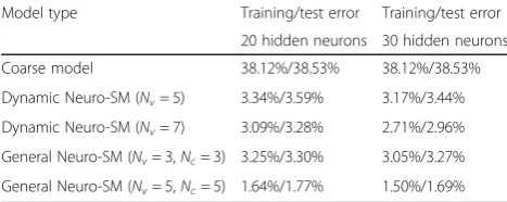
There are two important factors that impact the accur-acy of the dynamic Neuro-SM model and the proposed general Neuro-SM model, i.e., number of hidden

neurons and delay buffers. To show the results further, we compared the training and test error of the dynamic Neuro-SM and general Neuro-SM with different delay buffers and hidden neurons as shown in Table1. As seen

in Table 1, general Neuro-SM with 30 hidden neurons

and 5 delay buffers both for dynamic voltage and current mapping neural networks are suitable for this example.

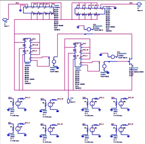
The proposed general Neuro-SM model can be conveniently implemented into the existing circuit simulators such as Keysight ADS for high-level

cir-cuit and system design. Figure 4 shows the proposed

general Neuro-SM model structure in ADS. The time delay parameter is 0.08 ns. In this figure, the dy-namic voltage mapping neural networks are embed-ded as the functions in two 7-port symbolically defined devices (SDDs), i.e., SDD7P1, and SDD7P2. Similarly, the dynamic current mapping neural net-works are embedded as the functions in two 9-port SDDs, i.e., SDD9P1 and SDD9P2. Time delay voltage and current signals can be obtained using voltage controlled voltage sources with delay parameters, i.e., SRC1~SRC8. After implementing the general Neuro-SM model into ADS, we have also compared simula-tion speed between coarse model, dynamic Neuro-SM, and the proposed general Neuro-SM model on an Intel i5-3230M 2.6 GHz computer as shown in

Table 2. The simulation was performed by Monte

Carlo analysis of 200 HB simulations. As seen in

Table 2, the simulation time is 48.32 s using coarse

model, compared to 57.17 s using general Neuro-SM, showing that the simulation speed of the pro-posed general Neuro-SM is acceptable in view of its good accuracy.

10 Conclusions

This paper has presented a general Neuro-SM tech-nique for nonlinear device modeling. By modifying the dynamic current and dynamic voltage relation-ships in the existing coarse model, the proposed gen-eral Neuro-SM model can exceed the accuracy limit over the coarse model, the Neuro-SM model with the

Table 1Training and test error comparison of coarse model, dynamic Neuro-SM model, and the proposed general Neuro-SM model after combined DC,Sparameter, and HB training

Model type Training/test error Training/test error

20 hidden neurons 30 hidden neurons

Coarse model 38.12%/38.53% 38.12%/38.53%

Dynamic Neuro-SM (Nv= 5) 3.34%/3.59% 3.17%/3.44%

Dynamic Neuro-SM (Nv= 7) 3.09%/3.28% 2.71%/2.96%

General Neuro-SM (Nv= 3,Nc= 3) 3.25%/3.30% 3.05%/3.27%

output mapping, and the dynamic Neuro-SM model. Compared to previously published Neuro-SM, the proposed general Neuro-SM has demonstrated much improved performance in terms of accuracy by a pHEMT modeling example. The general Neuro-SM model can be applied to microwave circuit and sys-tem design.

Acknowledgements

The authors would like to thank Prof. Q. J. Zhang at Carleton University, Ottawa, ON, Canada, for valuable discussions and insights throughout this work.

Funding

This work is supported by the Fundamental Research Funds for Universities in Tianjin (No. 2016CJ13), partly supported by the Key project of Tianjin Natural Science Foundation (No. 16JCZDJC38600), National Natural Science Foundation of China (No. 61601494, 61602346), and the Research Forums Cooperation Project of ZTE Corporation (2016ZTE04-09).

Availability of data and materials

The training and test data of the microwave transistor is obtained from measurement and can be shared if it is necessary.

Authors’contributions

The authors have contributed jointly to all parts on the preparation of this manuscript. LZ (first author) and JZ contributed to the structure and sensitivity analysis of the general Neuro-SM model. LZ (third author), WL and LP contributed to the training algorithm development. HW and DL contributed to the analysis of simulation results. All authors read and approved the final manuscript.

Competing interests

The authors declare that they have no competing interests.

Publisher’s Note

Springer Nature remains neutral with regard to jurisdictional claims in published maps and institutional affiliations.

Author details

1_{School of Control and Mechanical Engineering, Tianjin Chengjian University,} Tianjin 300384, China.2_{Tianjin Key Laboratory of Wireless Mobile}

Communications and Power Transmission, Tianjin Normal University, Tianjin 300387, China.3_{College of Electronic and Communication Engineering,} Tianjin Normal University, Tianjin 300387, China.4_{School of Microelectronics,} Tianjin University, Tianjin 300072, China.5_{Chengdu Ganide Technology Co.,} Ltd., Chengdu 610091, China.6_{Shijiazhuang Mechanical Engineering College,} Shijiazhuang 050003, China.

Received: 27 August 2017 Accepted: 20 January 2018

References

1. Z Li, Y Chen, H Shi, et al., NDN-GSM-R: a novel high-speed railway communication system via named data networking. EURASIP J. Wirel. Commun. Netw.48(1), 1–5 (2016)

2. H Shi, Z Li, D Liu, et al., Efficient method of two-dimensional DOA estimation for coherent signals. EURASIP J. Wirel. Commun. Netw.60, 1–10 (2017)

3. F Zhao, L Wei, H Chen, Optimal time allocation for wireless information and power transfer in wireless powered communication systems. IEEE Trans. Veh. Technol.65(3), 1830–1835 (2016)

4. D Liu, Z Li, X Guo, et al., DOA estimation for wideband chip with a few snapshots. EURASIP J. Wirel. Commun. Netw.28, 1–7 (2017)

5. F Zhao, B Li, H Chen, et al., Joint beamforming and power allocation for cognitive MIMO systems under imperfect CSI based on game theory. Wirel. Pers. Commun.73(3), 679–694 (2013)

6. F Zhao, W Wang, H Chen, et al., Interference alignment and game-theoretic power allocation in MIMO heterogeneous sensor networks

communications. Signal Process.126(9), 173–179 (2016)

7. Z Li, L Song, H Shi, Approaching the capacity of K-user MIMO interference channel with interference counteraction scheme. Ad Hoc Netw.58(4), 286–291 (2017) 8. F Zhao, H Nie, H Chen, Group buying spectrum auction algorithm for

fractional frequency reuses cognitive cellular systems. Ad Hoc Netw.58(4), 239–246 (2017)

9. F. Zhao, X. Sun, H. Chen, et al., Outage performance of relay-assisted primary and secondary transmissions in cognitive relay networks, EURASIP J. Wirel. Commun. Netw., 2014, 60(1).

10. L Zhang, J Xu, M Yagoub, et al.,Neuro-space mapping technique for nonlinear device modeling and large-signal simulation(IEEE MIT-S Int. Microwave Symp, Philadelphia, PA, 2003), pp. 173_–176

11. Q Zhang, K Gupta, V Devabhaktuni, Artificial neural networks for RF and microwave design: From theory to practice. IEEE Transaction on Microwave Theory and Techniques51(4), 1339–1350 (2003)

12. J Bandler, Q Cheng, S Dakroury, et al., Space mapping: the state of the art. IEEE Transaction on Microwave Theory and Techniques52(1), 337–361 (2004) 13. L Zhu, K Liu, Q Zhang, et al.,An enhanced analytical neuro-space mapping

method for large-signal microwave device modeling(IEEE MIT-S Int. Microwave Symp. Dig, Montreal, QC, 2012), pp. 1_–3

14. L Zhu, Q Zhang, K Liu, et al., A novel dynamic neuro-space mapping approach for nonlinear microwave device modeling. IEEE Microwave and Wireless Components Letters26(2), 131–133 (2016)

15. L Zhang, J Xu, MC Yagoub, et al., Efficient analytical formulation and sensitivity analysis of neuro-space mapping for nonlinear microwave device modeling. IEEE Transaction on Microwave Theory and Techniques53(9), 2752–2767 (2005)

16. Q Song, J Spall, Y Soh, et al., Robust neural network tracking controller using simultaneous perturbation stochastic approximation. IEEE Transaction on Neural Network19(5), 817–835 (2008)

17. Q Zhang, K Gupta,Neural network for microwave design(Artech House, Boson, MA, 2000)

18. L Zhang, QJ Zhang, Simple and effective extrapolation technique for neural-based microwave modeling. IEEE Microwave Component Letter20(6), 301– 303 (2010)

19. L Liu, J Ma, G Ng, Electrothermal large-signal model of III-V FETs including frequency dispersion and charge conservation. IEEE Transaction on Microwave Theory and Techniques57(12), 3106–3117 (2009)

20. NeuroModelPlus_V2.1E, Q. J. Zhang, Dept. of Electronics, Carleton University, Ottawa, ON, Canada.

Table 2Model simulation time comparison between coarse model, dynamic NEURO-SM, and the general Neuro-SM model

Model type HB simulation

Coarse model 48.32 s

Dynamic Neuro-SM 54.23 s