R E S E A R C H
Open Access
Numerical solution of stochastic
state-dependent delay differential equations:
convergence and stability
Bahar Akhtari
1**Correspondence: [email protected] 1Department of Mathematics, Institute for Advanced Studies in Basic Sciences (IASBS), Zanjan, Iran
Abstract
Numerical analysis of stochastic delay differential equations has been widely developed but frequently for the cases where the delay term has a simple feature. In this paper, we aim to study a more general case of delay term which has not been much discussed so far. We mean the case where the delay term takes random values. For this purpose, a new continuous split-step scheme is introduced to approximate the solution and then convergence in the mean-square sense is investigated. Moreover, given a test equation, the mean-square asymptotic stability of the scheme is presented. Numerical examples are provided to further illustrate the obtained theoretical results.
1 Introduction
In many physical phenomena with random nature, the state future of a system not only depends on the current state but also depends on the whole past history of the system over a finite time interval, and certainly the mathematical modelling actually describing the system leads to a stochastic delay differential equation (SDDE) and not a stochastic ordinary differential equation (SODE). In this paper, an autonomousd-dimensional Itô stochastic delay differential equation is considered
⎧ ⎨ ⎩
dX(t) =a(X(t),X(t–τ))dt+b(X(t),X(t–τ))dW(t), t∈[t0,T],
X(t) =η(t), t∈[t0–r,t0],
(1.1)
whereris a positive constant andτis calledlag process. The drift and diffusion coefficients
a,bj:Rd→Rdforj= 1, . . . ,mare Borel-measurable functions andη,η∈Rd, is named ini-tial process. Obviously, the inaccessibility of the closed-form of the solutions or their dis-tributions of these mathematical modelings, which arise in diverse areas of applications, reveal the significance of addressing numerical methods, because they play an important role to educe a realistic view of the solution behaviour of such equations. In recent years, some authors have dealt with the numerical analysis of SDDEs whose timelag is a dis-crete, see, e.g. [3,12,16]. But the delay function might be dynamically changed and even disturbed under an ambient noise. If the delay function depends only on time, then it is calledtime-dependent, see, e.g. [1,6,8,22]. But if, in addition to the time, it depends on the
solution process, then it is namedstate-dependent. As far as the author knows, only a few numerical schemes for SDDEs which contain the third type oflagfunction have been pro-posed, see, e.g. [13,14]. The authors [13,14] considered the continuous-timeGARCH(1, 1) model for stochastic volatility involving state-dependent delayed response and applied the Euler–Maruyama discrete-time approximation in the strong convergence sense to simu-late. On the other hand, there exist some papers which extend some types of stochastic functional (evolution, fractional, neutral) differential equations with state-dependent de-lay and study some theoretical aspects particularly the existence and uniqueness of (mild) solution and controllability results, see, e.g. [2,19,31,32]. In the following, a new interpo-lation, whose computational costs are not too high, is presented. The main contribution of this paper is to investigate the numerical solution of Eq. (1.1), under sufficient conditions which will be mentioned later, with three cases oflag processas follows:
(L1) τ is a constant,
(L2) τ is time-dependent asτ(t), (L3) τ is state-dependent asτ(t,X(t)).
Note that in case (L2),τcan be a continuous-time random process or a deterministic func-tion. Here, we just consider the deterministic case. Since the main task in all integration formulas for SDDEs is to provide an interpolation at non-mesh points, a new split-step scheme will be properly extended over the whole interval [t0,T]. The authors in [28] stud-ied the strong convergence and the mean-square stability of the split-step backward Euler method to linear SDDEs with constantlagand took the stepsize as a multiplier of that. This type of stepsize selection by a semi-implicit split-stepθ-Milstein method was developed in [7], too. But Wang et al. in [22] proposed a new improved split-step backward Euler method for SDDEs with time-dependent delay where a piecewise linear interpolation is used to approximate the solution at the delayed points. Also, in contrast to [7,28], in [22], the restriction of stepsize is removed and the unconditional stability property is extended as well. In our proposed method, this restriction on stepsize is dropped, too. As more pa-pers, we could mention [11,17] which investigate the behaviour of the split-type methods for stochastic differential equations and [26] which studies the strong convergence of the split-stepθ-method for a class of neutral stochastic delay differential equations.
As we know, the (numerical) stability concept is a powerful tool in measuring the sensi-tivity of the (difference) equation for any confusion. For instance, the disturbances, which occur during mathematical modelling, or round off errors made in the implementation of the numerical method may lead to fundamental changes. Undoubtedly, reviewing the numerical stability of stochastic differential equations is an inspiration to that of SDDEs. Among the most prominent papers which scrutinise the numerical stability for stochas-tic differential equations, the readers can refer to [9,20] for a review. Mao in [18] devel-opedpth moment and almost sure exponential stability of stochastic functional differen-tial equations by means of the Razumikhin-type theorems. Also, [25] examined almost sure exponential stability of the Euler–Maruyama scheme for such equations. Further-more, the authors in [4] employed the Halanay-type theory as the main tool to analyse
or SDDE with discrete or time-dependent delay [5,10,24,29,30], could be extended in the future. This paper consists of two parts. The first deals withconvergenceand the second withstability, both of which are examined in the mean-square sense.
This paper is organised as follows. Section2is concerned with the notations, assump-tions and a numerical scheme for the underlying problem. In Sect.3, the convergence of the scheme in the mean-square sense is derived. In Sect.4, we define the stability concept for the problem and numerical solution, too. Moreover, the mean-square stability of the scheme is established. Ultimately, some test problems are indicated in Sect.5.
2 Results formulation
Let (Ω,F,{Ft}t≥t0,P) be a complete probability space with the filtration{Ft}t≥t0satisfying
the usual conditions. Moreover,W= (Wt)t≥t0 is anm-dimensional Brownian motion on
the probability space. LetD=C([t0–r,t0],Rd) be the Banach space of all continuous func-tions from [t0–r,t0] toRd. Also, we use theLp(Ω,D) to be the space of allFt0-measurable
and integrable initial processesη:Ω→Dwhich can be equipped with the following semi-norm:
ηLp(D)=
Ω
ηpDdP
1/p
,
where the supremum norm · pDforp≥1 is defined as
ηpD= sup s∈[t0–r,t0]
η(s)p,
where| · |is the Euclidian norm inRk fork≥1. In this sequel, we make the necessary
assumptions on the problem as follows.
Assumption 1 The functionsa: (Rd)2→Rdandb: (Rd)2→Rd×mare globally Lipschitz continuous, i.e. there is a positive constantK1such that
a(X1,Y1) –a(X2,Y2) 2
∨b(X1,Y1) –b(X2,Y2) 2
≤K1 |X1–X2|2+|Y1–Y2|2
for allX1,X2,Y1,Y2∈Rd.
Assumption 2 In case (L2), letτ: [t0,T]→(0,r] be of Lipschitz continuous as
τ(t) –τ(s)≤K2|t–s|, t,s∈[t0,T],
whereK2is a positive constant. In case (L3), letτ : [t0,T]×Rd→(0,r] be of Lipschitz continuous, i.e. there exist two positive constantsK2andK3such that
τ(t,X) –τ(s,X)≤K2|t–s|, τ(t,X1) –τ(t,X2)≤K3|X1–X2|
Assumption 3 Given two adapted integrable stochastic processes ρ1,ρ2 : Ω ×[t0 –
r,T]→[t0–r,t0], we have
Eη ρ1(t)–η ρ2(s)2≤K4Eρ1(t) –ρ2(s), t,s∈[t0–r,T],
whereK4is a positive constant.
Theorem 2.1 Suppose that ηL2(D)<∞, under Assumptions 1–3, SDDE (1.1) has a unique strong solution X such that
XL2(D¯)≤H,
whereD¯ =C([t0–r,T],Rd)is the Banach space of all continuous sample paths with values
inRdand H is a positive constant.Moreover,there exists a positive constant K
5such that
for every t,s∈[t0,T]we have
EX ρ1(t)
–X ρ2(s) 2
≤K5Eρ1(t) –ρ2(s), (2.1)
whereρ1,ρ2:Ω×[t0,T]→[t0,T]are two adapted integrable stochastic processes.
The proof of the theorem above is deferred to theAppendix.
2.1 Underlying scheme
We now focus on the main intent, namely developing a new continuous split-step scheme based on the Euler–Maruyama to SDDE (1.1). To do this, consider a non-equidistant dis-cretization of the intervalI= [t0,T] as follows:
t0≤t1≤ · · · ≤tN=T,
the approximation X(t) for SDDE (1.1) is defined recursively through the underlying scheme
⎧ ⎪ ⎪ ⎨ ⎪ ⎪ ⎩
X(t0) =X∗(t0) =X(t0),
X∗(tk) =X(tk) +a(X∗(tk),Z(tk))tk, k= 1, . . . ,N– 1,
X(tk+1) =X∗(tk) +b(X∗(tk),Z(tk))Wk, k= 0, 1, . . . ,N– 1,
(2.2)
where iftk–τk≤t0, then
Z(tk) =η(tk–τk), (2.3)
otherwise iftk–τk∈[ti,ti+1), then
⎧ ⎨ ⎩
X∗(ti) =X(ti) +a(X∗(ti),Z(ti))((tk–τk) –ti),
Z(tk) =X∗(ti) +b(X∗(ti),Z(ti))(W(tk–τk) –W(ti)),
(2.4)
wheretk=tk+1–tkandWk=W(tk+1) –W(tk) are independent Gaussian distributed
random generation. Note thatτk in (2.3)–(2.4) is equal toτ andτ(tk) in cases (L1) and
(L2), respectively, and in case (L3),τk=τ(tk,X(tk)). One can simulate the valueW(tk–
τk) –W(ti) by means of the Brownian bridges to remain on the correct Brownian paths
[15]. We can extend the following continuous approximation for whole [t0,T]: ⎧
⎨ ⎩
X∗(ti) =X(ti) +a(X∗(ti),Z(ti))(t–ti),
Xi(t) =X∗(ti) +b(X∗(ti),Z(ti))(W(t) –W(ti)),
(2.5)
wheret∈[ti,ti+1) fori= 0, . . . ,N– 1. Furthermore,Z(ti) is obtained similar to (2.3)–(2.4).
We can present a continuous version of the approximation solution as follows:
X(t) =
N–1
i=0
Xi(t)1[ti,ti+1)(t) +X(tN)1{t=tN}, (2.6)
where 1 denotes the indicator function.
Proposition 2.2 Consider the approximation processes X∗,Z andX which are computed by(2.2), (2.3)and(2.4).Assume that a(0, 0) = 0and b(0, 0) = 0,then there exists a positive constantH such that¯
X∗L2(D¯)≤ ¯H, ZL2(D¯)≤ ¯H, XL2(D¯)≤ ¯H, (2.7)
whereD was specified in Theorem¯ 2.1.
In the sequel, for the simplicity, we takeH¯ such that it is equal toH in Theorem2.1. Under these conditions, we establish the strong convergence of scheme (2.5)–(2.6) over [t0,T] in the next section.
3 Convergence
Having been motivated to analyse the behaviour of scheme (2.5)–(2.6), we naturally con-centrate on the convergence concept. To this end, the mean-square convergence is invoked by a theorem as follows.
Theorem 3.1 Suppose that Assumptions1–3hold andηL2(D)<∞.Moreover,we assume that a(0, 0) = 0and b(0, 0) = 0.If we apply scheme(2.5)–(2.6)to SDDE(1.1),then
E
sup t0≤t≤T
e(t)2 1/2
=O hγ,
where e(t) =X(t) –X(t)and h=maxi=0,...,N–1ti.Moreover,γ is equal to1/2in cases(L1)
and(L2)and to1/4in case(L3).
Proof Note that proving of case (L1) is similar to that of (L2), so we leave it to the reader and we start proving with (L2). Lett∈[tn,tn+1). We can write
e(t) = t
t0
a X(s),X(s–τ)ds+ t
t0
b X(s),X(s–τ)dW(s)
– t
t0
a X∗(s),Z(s)ds– t
t0
where based on (2.5) and (2.6),X∗(s) =X∗(ti) andZ(s) =Z(ti) whens∈[ti,ti+1),i= 0, . . . ,n.
By Hölder’s and Doob’s martingale inequalities, we derive
E
By Assumption1, we have
whereZ(ti) =X(ti–τ(ti,X(ti))). We can writeA1i,A2i,A3iandA4iinstead ofA1,A2,A3 andA4to be more precise. But the second subscripts have been removed for the sake of simplicity. We now present the necessary upper bounds for these functions. Definitely
A1(s) = Ee(s)2. (3.2)
Due to the Hölder continuity property of the Brownian motion as well as Assumption1 and relation (2.7), we have Assumption3, Theorem2.1and due to being Lipschitz ofτin Assumption2, we see that
EX s–τ(s)–X ti–τ(ti)
Similar to the previous argument discussed in obtaining (3.4), we get
sinceNi=0–1ti=T–t0, the desired result is obtained. We now turn to case (L3) whereτ
Assumption3, Assumption2and Theorem2.1yield that
A31(s) = E1Ω1 X s–τ s,X(s)
by considering the dominant terms, we achieve
A31(s)≤K4K3 K5|s–ti|1/2+ Ee(ti).
We can write
In a similar manner which was employed in finding the upper bound ofA31(s), we see that
A32(s)≤2K3
The application of Gronwall’s lemma results in
whereC1=10(T3–t0)M(K4+K5)K3 √
K5e2M(T–t0). In view of (E(A))2≤E(A2), by Jensen’s in-equality, we can write
E
sup t0≤v≤t
e(v)2≤C1h1/2+ 9C1 10√K5
E
sup t0≤v≤t
e(v). (3.8)
We now set
A= E sup t0≤v≤t
e(v), (3.9)
and hence by (3.8) and (3.9)
A2≤C1h1/2+C2A,
whereC2=109√C1K
5. By recurrence, one sees that
A2≤C1h1/2+C2A
≤C1h1/2+C2
C1h1/2+C2A. (3.10)
We define
B=C1h1/2+C2A. (3.11)
By (3.10), firstly,
A2≤B, (3.12)
and secondly,
B≤C1h1/2+C2 √
B. (3.13)
SinceC2> 0 andA≥0, so from (3.11) we get
B–C1h1/2≥0. (3.14)
By (3.13) and (3.14), we observe that (B–C1h1/2)2≤C22Band
B2– C22+ 2C1h1/2
B+C12h≤0. (3.15)
For this quadratic inequality, we obtain two quantities forBas follows:
B1=
(C22+ 2C1h1/2) –
C24+ 4C1C22h1/2
2 ,
B2=
(C22+ 2C1h1/2) +
C24+ 4C1C22h1/2
Obviously, relation (3.15) is satisfied forB∈[B1,B2]. By the Taylor expansion of function
C24+ 4C1C22h1/2about pointC24, we achieve
B1=C12C24ξ2–3/2h,
B2=C22+C1 1 +C22ξ1–1/2
h1/2,
whereξ1,ξ2∈(C24,C24+ 4C1C22h1/2). By (3.12),A2≤Bfor allB∈[B1,B2] and alsoB1is the sharpest bound. Note that ifh→0, thenB1→0, and soA2→0. Hence, by definition
Ain (3.9), E(supt
0≤v≤t|e(v)|)→0, and we get E(supt0≤v≤t|e(v)|
2)→0 by (3.7). Henceforth,
the convergence of the scheme is visible. In order to determine a sharp bound forA2, we are interested in a quantity which is as small as possible. SoB1reveals the convergence rate. BecauseA=O(h1/2) and consequently by (3.9) and (3.7), we obtain
E
sup t0≤v≤t
e(v)2
=O h1/2.
Since there is no restriction ont, the desired result follows immediately.
Let us now mention two important remarks in line with Theorem3.1.
Remark3.2 ([21]) As we know, there exist no two seminorms which can be generally ma-jorized by a multiplier of each other. So there is no ambiguity if · L1 and · L2 are
proportional to different powers ofhin Theorem3.1.
Remark3.3 Note that as the scheme proceeds on the partitionΛ1to integrate the solution at the mesh points, whereΛ1={t0,t1, . . . ,tN =T}is a partition which covers all discrete
points, some points, which we can say are hidden, are brought up. For instance,tk∈Λ1 corresponds totk–τkand the approximationZk. We can renametk–τkbytmand make
partitionΛ2by means of these points. Besides, here, the underlying scheme and the in-terpolation, which approximate the stochastic process onΛ1andΛ2, respectively, are the same. So, practically, the proposed approximation computes the solution at the points in
Λ1andΛ2.
4 Stability
The main objective in the numerical stability literature is to examine whether the numeri-cal solution mimics the behaviour of the exact process or not. In particular, it is important to know the reaction of the scheme whenntends to infinity whilst the exact process be-comes trivial as large astbecomes very large. In fact, the impact of rounding errors, which are not inevitable, on the numerical results in the long term case is analysed. In this sec-tion, the asymptotic mean-square stability, corresponding to SDDE (1.1) and also a linear test equation, will be challenged.
Definition 4.1 The exact solution (strong solution) of SDDE (1.1) denoted byXis named asymptotically mean-square stable if
lim t→∞EX(t)
In the sequel, we present a theorem which deals with the mean-square stability of SDDE (1.1) and the proof sketch is given in theAppendix.
Theorem 4.2 Given SDDE(1.1)which satisfies Assumptions1–3,assume that there exist a positive constantλand non-negative constantsα0,α1,β0andβ1such that
xTa(x, 0)≤–λ|x|2,
a(x, 0) –a(x¯,y)≤α0|x–x¯|+α1|y|,
tracebT(x,y)b(x,y)≤β0|x|2+β1|y|2
for all x,x¯,y∈Rd.If
λ>α1+ 1
2(β0+β1),
then the zero solution is mean-square stable.
Definition 4.3 LetXbe the numerical solution of SDDE (1.1). If there existsh¯(a,b,c,d) > 0 such that the maximum stepsize lies in (0,h¯(a,b,c,d)), then the scheme is called asymp-totically mean-square stable if
lim
k→∞EX(tk)
2 = 0.
Theorem 4.4 Given SDDE(1.1),let Assumptions1–3hold andηL2(D)<∞.Assume that there exist two positive constantsλ1andλ2and non-negative constantsβ0andβ1such that
⎧ ⎨ ⎩
xTa(x,y)≤–λ
1|x|2+λ2|y|2,
trace[bT(x,y)b(x,y)]≤β
0|x|2+β1|y|2
(4.1)
for all x,y∈Rd.Assume that a(0, 0) = 0and b(0, 0) = 0.If2λ
1> 2λ2+β0+β1,β0λ2+β1λ1= 0
andtk∈(0,22(λ1β–20λλ22+–ββ10λ–1β)1),then scheme(2.2)–(2.4)is asymptotically mean-square stable.
Proof From (2.2), we can write ⎧
⎨ ⎩
|X(tk)|2=X∗(tk) –a(X∗(tk),Z(tk))tk,X∗(tk) –a(X∗(tk),Z(tk))tk
=|X∗(tk)|2– 2X∗T(tk)a(X∗(tk),Z(tk))tk+|a(X∗(tk),Z(tk))|2tk2,
by (4.1), we get
X(tk)
2
≥X∗(tk)
2
+ 2λ1X∗(tk)
2
–λ2Z(tk)
2
tk+a X∗(tk),Z(tk)
2
tk2
≥X∗(tk)
2
+ 2λ1X∗(tk)
2
–λ2Z(tk)
2
tk.
Henceforth, we get
X∗(tk)
2
≤ 1
1 + 2λ1tk X(tk)
2
+ 2λ2Z(tk)
2
tk
Again, from (2.2), we have
As it is customary, we consider a linear scalar test equation with state-dependent delay:
⎧
discrete delay and time-dependent delay can be found in [23,28]. The following corollary states what condition results in asymptotic mean-square stability for (4.3).
Corollary 4.5 If the following condition is satisfied
a< –|b|–(|c|+|d|) 2
2 , (4.4)
then SDDE(4.3)is mean-square stable.
Proof By Theorem4.2 and settingλ= –a,α0=|a|, α1=|b|, β0= 2|c|2, β1= 2|d|2, the
Now we turn our attention to the proposed method (2.2)–(2.4). Clearly, applying this scheme to the given equation (4.3) is indicated as
⎧
Remember that the scheme has been applied onΛ1, which is a non-uniform partition as
Λ1={t0,t1, . . . ,tN =T}, withtk =tk+1–tk andWk=Wk+1–Wk. Based on what was discussed in Remark3.3, we have an approximation onΛ1∪Λ2. This survey paves the way to analyse the stability of the scheme. In the following, the sufficient conditions to mean-square stability of scheme (4.5) will be determined.
Theorem 4.6 Under condition(4.4),the numerical scheme(4.5)applied to linear SDDE
(4.3)is asymptotic mean-square stable by some limitations on the stepsize.
Proof As we know, practically, the scheme proceeds along the partitionΛ1∪Λ2. Thus, we can write
Now, by applying the expectation, we have
E|Xk+1|2≤
we can rearrange the relation above as follows:
Note that based on what was discussed on the mesh points,tk–τk∈Λ2, and so we can
replaceZkwithXmin whichtm=tk–τk. Hence
E|Xk+1|2≤M(a,b,c,d,tk)·max
E|Xk|2, E|Xm|2
,
where
M(a,b,c,d,tk) =
1 +c2tk |1 –atk|2
1 + 2|b|tk+b 2
tk
2+ 2|dc|tk(1 +|b|tk) |1 –atk|
+d2tk.
Obviously, in order to have the desired result, we have to impose
M(a,b,c,d,tk) < 1, (4.6)
that is,tk must be selected such that M will be bounded by 1. Relation (4.6) yields that
1 +c2tk 1 + 2|b|tk+b 2
tk
2+ 2|dc|
tk 1 +|b|tk
|1 –atk|
+d2tk|1 –atk|
2<|1 –a
tk| 2,
and then
|cb|–|ad|2tk
2+ 2 |c|+|d| |cb|–a|d|+b2–a2
tk
+ 2a+ 2|b|+ |c|+|d|2< 0,
we now come up with a quadratic equation which can be invoked as
A(a,b,c,d)2+B(a,b,c,d)+C(a,b,c,d) < 0, (4.7)
with
A(a,b,c,d) = (ad)2– 2a|bcd|+ (bc)2,
B(a,b,c,d) = 2|c|+|d| |cb|–a|d|+b2–a2,
C(a,b,c,d) = 2a+ 2|b|+ |c|+|d|2.
We define
J(a,b,c,d,) =A(a,b,c,d)2+B(a,b,c,d)+C(a,b,c,d).
Here, we first consider
J(a,b,c,d,) = 0, (4.8)
and compute the discriminantfor that. Obviously,A(a,b,c,d)≥0 and by Theorem4.5 we have
It follows that≥0 with
=B(a,b,c,d)2– 4A(a,b,c,d)C(a,b,c,d).
If A(a,b,c,d) > 0, then the discriminant is positive, and we have two distinct roots
h1(a,b,c,d) andh2(a,b,c,d). Furthermore, given the relation between the roots of a poly-nomial and its coefficients, we get
h1(a,b,c,d)∗h2(a,b,c,d) =C(a,b,c,d)
A(a,b,c,d)< 0.
It is profitably viewed that h1(a,b,c,d) and h2(a,b,c,d) have different signs. Without any loss of generality, we assume that h1(a,b,c,d) <h2(a,b,c,d), then (4.7) is satisfied for all tk ∈ (h1(a,b,c,d),h2(a,b,c,d)). Hence, if the stepsize is taken in the interval (0,h2(a,b,c,d)), then the stability of the scheme will be guaranteed. IfA(a,b,c,d) = 0, then
B(a,b,c,d) =b2–a2 and by Theorem4.5,b2<a2, and soB(a,b,c,d) < 0. In this case, for all stepsizes, relation (4.7) is satisfied, and so unconditional stability arises. So we can say iftk∈(0,h¯) for allk, whereh¯=∞orh¯=h2(a,b,c,d), scheme (4.5) is asymptotic
mean-square stable.
Remark4.7 We can prove Theorem4.6using Theorem4.4by settingλ1= –a–|b|2,λ2=|b|2,
β0=|c|2+|c||d|andβ1=|d|2+|c||d|. By (4.4), we have 2λ1> 2λ2+β0+β1 andβ0λ2+
β1λ1= 0. By Theorem4.4, if we take the stepsize in (0,h∗),h∗= –2a–2|b|–(|c|+|d|)
2
|b|(|c|2+|cd|)+(|d|2+|cd|)(–2a–|b|),
then scheme (4.5) is mean-square stable. Thus, iftk∈(0,h˜) for allk, then scheme (4.5) is mean-square stable whereh˜=max(h∗,h¯). Note thath¯was obtained in the proof of Theo-rem4.6.
5 Simulation experiments
In this section, we seek the accuracy and efficiency of the numerical scheme for some test problems. As we know, stochastic models in addition to the deterministic aspect possess a probabilistic one. Accordingly, the noise process must be properly simulated in order to obtain an efficient numerical scheme. In this work, the Wiener process models the noise, and one must be careful when generating the Brownian motion and take an approach such that the correct paths of that are followed. Particularly, due to the delay nature, some points become evident during the implementation of the scheme which do not belong to the partition but have to be simulated. For this aim, given the Markov property of the Wiener process, one can utilise a linear interpolation to simulateWtif the valuesWt1and Wt2,t1<t<t2, are known. We callWti,Wti=Wti+1–Wti, to be the Brownian increment andti,ti=ti+1–ti, to be time one. Besides, one very challenging point in the study of
Example5.1 ⎧ ⎨ ⎩
dX(t) = (–3X(t) + 0.5X(t– 1))dt+ (X(t) +X(t– 1))dW(t), t∈[0,T],
η(t) = 1 +t, t∈[–1, 0].
Here τ = 1 and in the determining the parameters, the numerical stability condition has been taken into account, see relation (4.4), and such condition will also be considered in the two next examples. Since delay is constant, for everyti,ti– 1 point situates in a
subinterval far from current interval, and accordingly theoverlappingdoes not exist. We postpone this discussion to the next example. Consequently, the relevant programmes are easily accomplished, which leads us to Table1, Fig.1and Fig.5.
As a second problem, we consider the time-dependent case with a delay function (1 +
t2)–1decreasing versus time.
Example5.2 ⎧ ⎨ ⎩
dX(t) = (–4X(t) +X(t–1+1t2))dt+ (X(t) +X(t–1+1t2))dW(t), t∈[0,T],
η(t) = 1, t∈[–1, 0].
By virtue of the fact that (1 +t2)–1decreases int, it is expected that the implementation of the scheme with a slight difference is similar to (L1). Here, unlike the constant delay, we face overlapping. We use the word overlapping if during the implementation of the scheme, there exists a pointti+1such thatti+1–τi+1∈[ti,ti+1) separates the latter interval
into [ti,ti+1–τi+1) and [ti+1–τi+1,ti+1). In this case, by approximating the process atti+1–
τi+1, because of the fact that the scheme is one-step, recomputation ofX(ti+1) is required. So the generation of each path is more time-consuming than that of the previous one. Furthermore, stepsize 2–12will be selected to create a partition in order to simulate the exact solution in these two examples.
Example5.3
⎧ ⎪ ⎪ ⎨ ⎪ ⎪ ⎩
dX(t) = (–5X(t) +X(t–c|X+|X(t()t|)|))dt
+ (0.5X(t) +X(t–c+|X|X(t()t|)|))dW(t), t∈[–1,T],
X(t) = 0.5, t≤–1,
whereτ(t,X(t)) =c+|X|X(t()t|)|, and letcbe a positive constant.
Here, according to the dependence of the delay term on the noise process, the simulation is not analogous to the two previous ones. Notice that for every pointti, in addition toXi,
the amountZihas to be computed, namely approximation of the process atti–τi, and if we
denote this point bytmi, then the valueZmihas to be computed. If we settki=tmi–τmi, then
an important question is whether the quantityZkihas to be computed or not. Since in the
two first cases of delay term we havetmj>tmi>tkifor everyjsuch thatj>i, so we do not
need the approximationZki. Note thatτis a decreasing function in Example5.2. Hence, in
constant. But in the state-dependent case, as we evidently observed in our running, unlike the two first cases, going back to the past is not necessarily consecutive. Hence, we might useZkiduring the next computations, and so it has to be modified. Assume that nesting
calculations have to be required at the pointstki1<tki2<· · ·<tkil<tki, and naturally they have to be stopped after a finite period. For this, we rectifyZki1by averaging everyZjwhere
Zj=αforj<ki1. By the way, the overlapping problem exists here, too. Thus, as mentioned in the previous example, we must carefully execute the scheme. Considering the case of state-dependent delay which includes more computation errors, too many small stepsizes may lead us to a wrong direction. So our proposed partition is made by the stepsize 2–11. Needless to say, time and computing costs are considerably higher than those of the two previous cases.
5.1 Comment on results
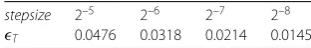
After having finished implementing the numerical scheme for the three examples above, we now hint at some tips in line with the obtained numerical results. To simplify the nota-tion, letXeandXastand for the exact and numerical solutions, respectively. The numer-ical implementations have been made with various input stepsizes up to the end of the interval and the exact one by a small stepsize as previously mentioned forNdiscretized Brownian paths. Then, in order to visualise errorT= E|Xe(T) –Xa(T)|inspiring
confi-dence to the scheme, practically, we utilise the sample mean of the individual paths as 1
N
N
i=1|Xie(T) –Xia(T)|providedN is sufficiently large. Here,N= 10,000. All four
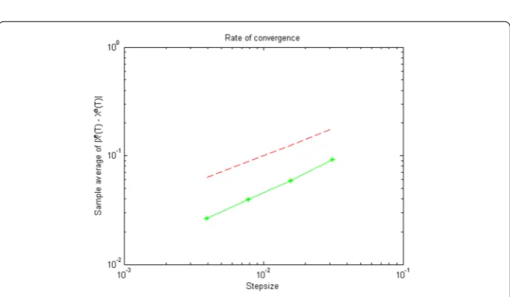
Ta-bles1,2,3and4reveal the reasonable behaviour of the computational error to the shrink-aging of the stepsize. Apparently, the smaller stepsize results in improving the approxima-tion, which indicates the significant response of the scheme. In order to indicate the speed of convergence of the scheme, we draw the logarithm of global computational error versus that of the stepsize. In doing so, the commandloglogin Matlab, which is interpreted as the logarithm function, has been applied and it provides us with Figs.1,2,3and4. We observe that the obtained curves are parallel to the functionsx12andx14, which is in agreement with
Table 1 Computational error at endpointT= 1 for Example5.1
stepsize 2–5 2–6 2–7 2–8
T 0.0476 0.0318 0.0214 0.0145
Table 2 Computational error at endpointT= 1 for Example5.2
stepsize 2–5 2–6 2–7 2–8 T 0.0917 0.0590 0.0394 0.0266
Table 3 Computational error at endpointT= 1 for Example5.3withc= 0.01
stepsize 2–5 2–6 2–7 2–8
T 0.1619 0.1374 0.1181 0.1017
Table 4 Computational error at endpointT= 1 for Example5.3withc= 1
Figure 1The rate of strong convergence for Example5.1withT= 1. The logarithm ofTis denoted by the
green line with asterisk which is parallel with the dashed red line by slope12
Figure 2The rate of strong convergence for Example5.2withT= 1. The logarithm ofTis denoted by the
green line with asterisk which is parallel with the dashed red line by slope12
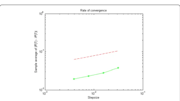
the theoretical results. Remember that we must pay particular attention to (4.4) in order to preserve the numerical stability. The parameters of the given problem areT= 20 and
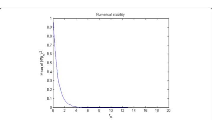
ti= 0.2. Note that Figs.5,6,7and8present the mean of normed approximation over N realisations as N1 Ni=1|Xa
i(tn)|2, which establishes the stability. Regarding the trends,
one can see that the summation converges to zero astnbecomes larger. By means of these
results, we conclude that scheme (2.2)–(2.4) is a well-developed scheme for problem (1.1).
6 Conclusion
Figure 3The rate of strong convergence for Example5.3withT= 1,c= 0.01. The logarithm ofTis denoted
by the green line with asterisk which is parallel with the dashed red line by slope14
Figure 4The rate of strong convergence for Example5.3withT= 1,c= 1. The logarithm ofTis denoted by
the green line with asterisk which is parallel with the dashed red line by slope14
Figure 5The average of numerical solution over 10,000 discretized Brownian paths withh= 0.2 andT= 20 for Example5.1
Figure 6The average of numerical solution over 10,000 discretized Brownian paths withh= 0.2 andT= 20 for Example5.2
Appendix: Proofs
In this section, we deal with proving Theorems2.1and4.2. First, we start with a useful lemma.
Lemma A.1 Assume that X,Y:Ω → ¯D are two stochastic processes with D¯ =C([t0–
r,T],Rd).Furthermore,X and Y are denoted byηXandηYon[t0–r,t0],respectively.
Con-sider the functionτ which has been defined in Assumption2and suppose that there exists a positive constant H such that
Figure 7The average of numerical solution over 10,000 discretized Brownian paths withh= 0.2,T= 20 and c= 0.01 for Example5.3
Figure 8The average of numerical solution over 10,000 discretized Brownian paths withh= 0.2,T= 20 and c= 1 for Example5.3
Then there exists a positive constant L∗such that,for all t∈[t0,T],
EX t–τ t,X(t)–Y t–τ t,Y(t)2
≤L∗
E
sup t0≤s≤t
X(s) –Y(s)2
+ηX–ηY2L2(D)
, (A.2)
where D=C([t0–r,t0],Rd).
Proof We divide [t0,T] into two sets as follows:
I1=
t∈[t0,T];PX(t)=Y(t)= 0,
I2=
For allt∈I1, we can easily write
EX t–τ t,X(t)–Y t–τ t,Y(t)2
≤E
sup t0≤s≤t
X(s) –Y(s)2
+ηX–ηY2L2(D)
,
ift∈I2, then we define
Lt=
E|X(t–τ(t,X(t))) –Y(t–τ(t,Y(t)))|2
E|X(t) –Y(t)|2+η
X–ηY2L2(D)
.
We claim thatLtis bounded above. If we suppose that the claim is not true, then for every
α> 0 there existstα∈I2such thatLtα>αand
EX tα–τ tα,X(tα)
–Y tα–τ tα,Y(tα) 2
>α EX(tα) –Y(tα) 2
+ηX–ηY2L2(D)
,
clearly, due to (A.1), E|X(tα) –Y(tα)|2+ηX–ηY2L2(D)≤4H2, and so the right-hand side
of the expression above will tend to infinity asα→ ∞, i.e.
EX tα–τ tα,X(tα)
–Y tα–τ tα,Y(tα) 2
→ ∞.
Also, by (A.1) again, for allα> 0,
EX tα–τ tα,X(tα)
–Y tα–τ tα,Y(tα) 2
≤2H2.
These two last expressions reveal a contradiction. Therefore, the claim is true and we can set
¯
L=sup t∈I2
Lt.
Finally, we obtain
EX t–τ t,X(t)–Y t–τ t,Y(t)2
≤ ¯L EX(t) –Y(t)2+ηX–ηY2L2(D)
≤ ¯L
E
sup t0≤s≤t
X(s) –Y(s)2
+ηX–ηY2L2(D)
,
wheret∈I2. By settingL∗=max{¯L, 1}, the desired result is obtained.
In the sequel, we define a unique strong solution for SDDE (1.1) in the third case.
Definition A.2 The stochastic processXis called a strong solution of SDDE (1.1) in case (L3) if the following properties are satisfied:
2. For allt≥0, with probability one we have tions above, then we say the solution satisfies the uniqueness.
Now we deal with the proving of Theorem2.1. Since there exist some texts which deal with the existence and uniqueness for cases (L1) and (L2), so we just consider the third case.
Proof of Theorem2.1 First, supposing that the equation has a strong solutionX, we show that XL2(D¯)<∞, and thenX is unique in the strong sense. Finally, we deal with the
By Gronwall’s inequality, we get
Note thatH> 0. In order to prove the Hölder type of the exact solution, we suppose that, for every positive constantα> 0, there existtα,sα∈[t0,T] such that bounded random variables taking values in [t0,T]. In addition, from (A.4) we have
E|X(ρ1(tα)) –X(ρ2(sα))|2≤2H2. So it is a contradiction, and then there exists a positive constant, likeK5, such that (2.1) holds.
Now we firstly prove the uniqueness and secondly the existence. Suppose thatXandY
are the two strong solutions of the equation withY(s) =X(s) =η(s) for alls∈[t0–r,t0].
by Assumption1, Hölder’s and Doob’s inequalities
≤3Eη(t0)2+ 18 (t–t0) + 4K1(t–t0)η2L2(D)
for everyk≥1. By Gronwall’s lemma, we get
max
sequenceXn(t) is convergent. Corresponding to (A.6) and by Assumption1, Hölder’s and
Doob’s inequalities
and Doob’s inequalities and also Assumption1
E
Analogously, one can see that, for alln≥1,
E
Hence, by Chebyshev’s inequality, we get
whered= 2bK1(1 +L∗)(T–t0). It is clear that∞n=0dnn! <∞, and so by the Borel–Cantelli lemma, for almost allω∈Ω, there existsn0=n0(ω), which is a positive integer such that
sup t0≤v≤T
Xn+1(v) –Xn(v)2≤ 1
2n, n≥n0.
Hence, for allt∈[t0,T],
Xn(t) =X0(t) +
n
i=1
Xi+1(t) –Xi(t),
since |Xi+1(t) –Xi(t)|< 1 (√2)i and
n i=1
1
(√2)i is convergent, so by a sufficient condition presented by K. Weierstrass,Xn(t) converges uniformly. We setX(t) =limn→∞Xn(t). By (A.12), we can find that Xn(t) is a Cauchy sequence. So, for everyε> 0, there exists n0(ε)∈Nsuch that, for alln≥n0(ε), we have
E
sup t0≤u≤t
Xn(u) –X(u)2
≤ε,
so by (A.9), E(supt0≤u≤t|X(u)|2)≤ ¯H. Notice that item 2 in DefinitionA.2is satisfied and, obviously,Xis continuous and adapted. Now we must examine whetherX(t) is satisfied in problem (1.1). By Assumptions 1and2, one can see thatτ(t,Xn(t)), a(Xn(s),Xn(s–
τ(s,Xn(s)))) andb(Xn(s),Xn(s–τ(s,Xn(s)))) converge pointwise toτ(t,X(t)),a(X(s),X(s–
τ(s,X(s)))) andb(X(s),X(s–τ(s,X(s)))), respectively. By Assumption1and relation (A.9), we apply the dominated convergence theorem, and so
t
t0
a Xn(s),Xn s–τ s,Xn(s)ds−→
t
t0
a X(s),X s–τ s,X(s)ds, t
t0
b Xn(s),Xn s–τ t,Xn(s)dW(s)−→ t
t0
b X(s),X s–τ s,X(s)dW(s),
where the convergence occurs in probability. Hence
Xn(t0) + t
t0
aXn(u),Xn u–τ u,Xn(u)du
+ t
t0
b Xn(u),Xn u–τ u,Xn(u)dW(u),
with probability one tending to
X(t0) + t
t0
a X(u),X u–τ u,X(u)du+ t
t0
b X(u),X u–τ u,X(u)dW(u).
We now deal with the proof of Theorem4.2. The proof in the two first cases, whereτ
Theorem A.3 Consider SDDE(1.1)with state-dependent delay satisfying Assumptions1–
3.Suppose that there exists a function V: [t0–r,∞)×Rd→R+which is continuous once
differentiable with respect to the first variable and twice to the second one.Besides
c1|x|p≤V(t,x)≤c2|x|p, (t,x)∈[t0–r,∞)×Rd, (A.13)
where c1,c2,p> 0,and there exists positive constantλ1such that,for all t≥0,
E L V(t,η)≤–λ1EV t,η(t0)
, (A.14)
whenever we have
E V t+θ,η(t0+θ)
<λ0EV t,η(t0)
, (A.15)
whereλ0> 1.Also,ηis a stochastic process which was defined in Sect.2.Furthermore,θ
is a random variable taking values in[–r, 0].Notice that operatorL:C1,2([t
0–r,∞)×
Rd,R+)→Ris given as ⎧
⎪ ⎪ ⎨ ⎪ ⎪ ⎩
L(V(t,η)) =∂V(t,η(t0))
∂t +
d
i=1ai(η(t0),η(–τ(t,η(t0))))∂V(∂t,xηi(t0)) +12dk,l=1mj=1bk,j(η(t0),η(–τ(t,η(t0)))) ×∂2V(t,η(t0))
∂xl∂xk b
l,j(η(t0),η(–τ(t,η(t0)))).
(A.16)
Then
EX(t)p≤Ke–γt, t≥t0,
with K=c2
c1Eη
pandγ =min(λ1,log(λ0)
r ).
Proof We define
U(t) = E
max θ∈[–r,0]e
¯
γ(t+θ)V t+θ,X(t+θ), t≥t0, (A.17)
whereγ¯ =γ – for as an arbitrary positive constant and alsoθ is a random variable taking values in [–r, 0]. We suppose that the maximum occurs inθ¯, that is,
U(t) = E eγ¯(t+θ¯)V t+θ¯,X(t+θ¯). (A.18)
Note thatU(t)≥0. We claim thatU(t) <U(t0). For this aim, we show thatUis a decreasing function. Clearly, for all random variablesθ∈[–r, 0],
E eγ¯(t+θ)V t+θ,X(t+θ)≤U(t).
Here, we review two casesθ¯= 0 andθ¯= 0. Ifθ¯= 0 almost surely, then by (A.17)
for all random variablesθ∈[–r, 0]. By relations (A.13) and (A.19), we havec1E(eγ¯(t+θ)|X(t+
θ)|p)≤E(eγ¯tV(t,X(t))). IfU(t), namely E(eγ¯tV(t,X(t))), is equal to zero, then almost surely
X(t+θ)p= 0 (A.20)
for all random variablesθ∈[–r, 0]. We assert thatU(t+h) = 0 for every sufficiently smallh. IfU(t+h) > 0, then there exists a random variableθ∗such that
U(t+h) = E eγ¯(t+h+θ∗)V t+h+θ∗,X t+h+θ∗,
it is clear that E(eγ¯(t+h+θ∗)V(t +h+θ∗,X(t+h+θ∗))) > 0. Due to the continuity of
E(eγ¯·V(·,X(·))) and sincehis a very small quantity, we have E(eγ¯(t+θ∗)V(t+θ∗,X(t+θ∗))) >
0. Moreover, by relation (A.13),X(t+θ∗)= 0 almost surely and it is a contradiction with (A.20). So the assertion is true, i.e.U(t+h) = 0 andU(t+h)≤U(t). We now turn to the caseU(t) > 0, that is, E(eγ¯tV(t,X(t))) > 0. By (A.19), we have
E eγ θ¯ V t+θ,X(t+θ)≤E V t,X(t),
it is obvious that
E e–γ¯rV t+θ,X(t+θ)≤E V t,X(t),
by settingλ0=eγ¯r andη(t0+θ) =X(t+θ), relation (A.15) is satisfied. Accordingly, by (A.14), we achieve
E L V(t,η)≤–λ1EV t,X(t)
,
whereη(t0) =X(t). So we can write
E eγ¯(t+h)V t+h,X(t+h)– Eeγ¯tV t,X(t)= t+h
t
eγ¯sγ¯E V s,X(s)
+eγ¯sEL V s,X(s)ds
≤ t+h
t
eγ¯s(γ¯–λ
1)E V s,X(s)
ds
≤0
for everyh> 0. So
E eγ¯(t+h)V t+h,X(t+h)≤E eγ¯tV t,X(t). (A.21)
We claim that U(t+h) = E(eγ¯(t+h)V(t+h,X(t+h))) for every sufficiently smallh> 0. It means that the maximum in (A.17) takes place in θ∗= 0 almost surely. Assume that it does not hold, thenU(t+h) = E(eγ¯(t+h+θ∗)V(t+h+θ∗,X(t+h+θ∗))) withP{θ∗< 0}> 0,
and so, for all random variablesθ∈[–r, 0],
Due to the continuity of E(eγ¯·V(·,X(·))), we obtain
E eγ¯(t+θ)V t+θ,X(t+θ)≤Eeγ¯(t+θ∗)V t+θ∗,X t+θ∗,
and especially forθ= 0 almost surely
E eγ¯tV t,X(t)≤E eγ¯(t+θ∗)V t+θ∗,X t+θ∗,
but it disaffirms (A.19). So the claim is satisfied, and by (A.21) we getU(t+h)≤U(t). We now turn to the caseP{ ¯θ< 0}> 0. We claim thatU(t+h)≤U(t) for every sufficiently small
h> 0. If
⎧ ⎨ ⎩
U(t+h) = E(eγ¯(t+h+θ∗)V(t+h+θ∗,X(t+h+θ∗))),
U(t+h) >U(t).
Due to the continuity of E(eγ¯·V(·,X(·))), we obtain
E eγ¯(t+θ∗)V t+θ∗,X t+θ∗>U(t). (A.22)
We observe that (A.22) contradicts (A.18), and so the claim is satisfied. Based on what was discussed above, we arrive atU(t+h)≤U(t) for every sufficiently smallh. Now we define Dini-derivativesD+U(t) as
D+U(t) =lim sup h→0+
U(t+h) –U(t)
h .
ConsideringD+U(t)≤0, the functionUis non-increasing, see Lemma 5 in [4]. SoU(t)≤
U(t0). Putting everything together, we get
E eγ¯tV t,X(t)≤E eγ¯(t+θ¯)V t+θ¯,X(t+θ¯)
≤E
max θ∈[–r,0]e
¯
γ(t0+θ)V θ+t0,X(θ+t0),
since|eγ θ¯ | ≤1 and by (A.13), we obtain
c1eγ¯tE X(t)
p
≤c2eγ¯t0E
max θ∈[–r,0]
η(t0+θ)
p
.
Consequently,
EX(t)p≤c2
c1
e–γ¯(t–t0)Eηp.
Theorem A.4 Assume that Assumptions1–3are fulfilled.Consider the function V defined in TheoremA.3holding condition(A.13).Moreover,for all t≥0and x,y∈Rd,
∂V(t,x)
∂t +
d
i=1
ai(x,y)∂V(t,x)
∂xi
+1 2
d
k,l=1
m
j=1
bk,j(x,y)∂ 2V(t,x)
∂xl∂xk
bl,j(x,y)
≤–λV(t,x) +λ¯V t–τ(t,x),y, (A.23)
whereλandλ¯are positive constants.Remember thatτ is the lag function.Ifλ>qλ¯ for all q∈(1,λ/λ¯),then the zero solution of SDDE(1.1)with state-dependent delay is pth moment exponentially stable.
Proof The proof starts with reviewing the condition in the previous theorem. Just check-ing relation (A.14) is required. In relation (A.23) we setx=η(t0) andy=η(–τ(t,η(t0))), so
∂V(t,η(t0))
∂t +a η(t0),η –τ t,η(t0)
∂V(t,η(t0))
∂x
+1 2b
T η(t0),η –τ t,η(t0)∂2V(t,η(t0))
∂x2 b η(t0),η –τ t,η(t0)
≤–λV t,η(t0)+λ¯V t–τ t,η(t0),η –τ t,η(t0). (A.24)
We can call the left-hand side (A.24) byL(V(t,η)), and so
E L V(t,η)≤–λE V t,η(t0)
+ E λ¯V t–τ t,η(t0)
,η –τ t,η(t0)
.
If we suppose that
E V t–τ t,η(t0),η–τ t,η(t0)≤qE V t,η(t0), forq∈(1,λ/λ¯),
then
E L V(t,η)≤(–λ+qλ¯)E V t,η(t0),
so the proof is complete.
Finally, next theorem concludes our aim.
Theorem A.5 Consider SDDE(1.1)with state-dependent delay which satisfies Assump-tions1–3.Assume that there exist a positive constantλand non-negative constantsα0,α1,
β0andβ1such that
xTa(x, 0)≤–λ|x|2,
a(x, 0) –a(x¯,y)≤α0|x–x¯|+α1|y|,