© 2015, IRJET.NET- All Rights Reserved
Page 1854
An Efficient Differential Evolutionary approach to Optimal Reactive
Power Dispatch with Voltage Profile Improvement
Mr. Bhaskar Mahanta
1,
Dr. Barnali Goswami
21
P.G. Research scholar, Electrical Engineering Department, Assam Engineering College, Assam, India
2Associate Professor, Electrical Engineering Department, Assam Engineering College, Assam, India
---***---Abstract -
In any power system faults occur due tounexpected outages of lines or transformers or other disturbances which are referred to as contingencies may cause voltage instability in the power system. Reactive power plays a very important role in the power system. In a power system when reactive power absorbed is greater than reactive power generated, the system voltage falls from its normal operating value and system voltage rises from its normal operating range when reactive power generated is greater than reactive power absorbed. Therefore optimization of reactive power dispatch and maintaining voltage at the load buses are two important tasks to be performed in a power system. This paper proposes an efficient differential evolutionary algorithm (DEA) to solve the optimal reactive power dispatch (ORPD) problems. The main objective of optimal reactive power dispatch is to minimize the real power loss with the optimal setting of the control variables. The continuous control variables are-generator bus voltage magnitudes and the discrete control variables are-transformer tap settings. The proposed approach employs differential evolution algorithm for optimal setting of reactive power dispatch control variables. The differential evolution solution has been tested on two standard IEEE systems. i.e. 14 and 30 bus test systems to minimize the total active power loss and to improve the voltage profile.
Key Words:
Active Power loss, Differential Evolution
Algorithm, Reactive power, Voltage Profile, etc…
1. Introduction:
The purpose of the reactive power dispatch (RPD) in power system is to identify the control variables which minimize the given objective function while satisfying the unit and system constraints. This goal is achieved by proper adjustment of reactive power variables like generator voltage magnitudes and transformer tap
setting. The main objective of optimal reactive power control is to improve the voltage profile and minimizing system real power losses via redistribution of reactive power in the system. To solve the RPD problem, a number of conventional optimization techniques [1, 2] have been proposed. These include the Gradient method, Non-linear Programming (NLP), Quadratic Programming (QP), Linear programming (LP) and Interior point method. Though these techniques have been successfully applied for solving the reactive power dispatch problem, still some difficulties are associated with them. One of the difficulties is the multimodal characteristic of the problems to be handled. Also, due to the non-differential, non-linearity and non-convex nature of the RPD problem, majority of the techniques converge to a local optimum. Recently, Evolutionary Computation techniques like Genetic Algorithm (GA) [3], Evolutionary Programming (EP) [4] and Evolutionary Strategy [5]have been applied to solve the optimal dispatch problem. In this paper, a new evolutionary computation technique, called Efficient Differential Evolution (DE) algorithm is used to solve RPD problem. The DE [6] has three main advantages: it can find near optimal solution regardless the initial parameter values, its convergence is fast and it uses few number of control parameters. In addition, DE is simple in coding and easy to use. It can handle integer and discrete optimization. The performance of DE algorithm was compared to that of different heuristic techniques. It is found that, the convergence speed of DE is significantly better than that of GAs [7].
© 2015, IRJET.NET- All Rights Reserved
Page 1855
2. Problem Formulation:
The objective of RPD is to identify the reactive power control variables, which minimizes the objective functions stated as follows:
2.1 Minimization of system power losses:
The minimization of system real power losses Ploss (MW) can be calculated as follows:
where nl is the number of transmission lines; is the conductance of the kth line; and are the voltage magnitude at the end buses i and j of the kth line, respectively, and and are the voltage phase angle at the end buses i and j.
2.2 Voltage profile improvement:
Bus voltage is one of the most important security and service quality indices. Improving voltage profile can be obtained by minimizing the load bus voltage deviations from 1.0 per unit. The objective function can be expressed as:
Where is the number of load buses.
2.3. System Constraints:
2.3.1. Equality constraints:
These constraints represent load flow equations:
where i=1,. . .,NB; NB is the number of buses, is the active power generated, is the reactive power generated, is the load active power, is the load reactive power, and are the transfer conductance and susceptance between bus i and bus j, respectively.
2.3.2. Inequality Constraints:
These constraints include:
1. Generator constraints: generator voltages, and reactive power outputs are restricted by their lower and upper limits as follows:
2. Transformer constraints:
Transformer tap settings are bounded as follows:
Security constraints:
These include the constraints of voltages at load buses and transmission line loadings as follows:
By adding the inequality constraints to the objective function, the augmented fitness function to be minimized becomes:
Where , and are the penalty factors, these penalty factors are large positive constants. is the number of load buses (PQ buses) and nbr is the total number of transmission lines.
3. Differential Evolution Algorithm:
3.1. Overview:
In 1995, Storn and Price proposed a new floating point encoded evolutionary algorithm for global optimization and named it differential evolution (DE) algorithm owing to a special kind of differential operator, which they invoked to create new off-spring from parent chromosomes instead of classical crossover or mutation.
© 2015, IRJET.NET- All Rights Reserved
Page 1856
parents. DE employs a greedy selection process that is thebest new solution and its parent wins the competition providing significant advantage of converging performance over genetic algorithms.
Fig 3.1:
DE cycle of stages3.2. DE computational flow:
DE algorithm is a population based algorithm using three operators; crossover, mutation and selection. Several optimization parameters must also be tuned. These parameters have joined together under the common name control parameters. In fact, there are only three real control parameters in the algorithm, which are differentiation (or mutation) constant F, crossover constant CR, and size of population NP. The rest of the proper setting of NP is largely dependent on the size of the problem. Storn and Price remarked that for real-world engineering problems with D control variables, NP=20D will probably be more than adequate, NP as small as 5D is often possible, although optimal solutions using NP<2D should not be expected. Storn and Price set the size of population less than the recommended NP=10D in many of their test tasks. It is recommended using of NP≥4D. NP=5D is a good choice for a first try, and then increase or decrease it by discretion. So, as a rough principle, several tries before solving the problem may be sufficient to choose the suitable number of the individuals. The DE algorithm works through a simple cycle of stages, presented in Fig.3.1. These stages can be cleared as follow:
3.2.1. Initialization:
At the very beginning of a DE run, problem independent variables are initialized in their feasible numerical range. Therefore, if the jth variable of the given problem has its lower and upper bound as and , respectively, then the jth component of the ith population members may be initialized as:
where , rand(0,1) is a uniformly distributed random number between 0 and 1.
3.2.2. Mutation:
In each generation to change each population member _Xi(t), a donor vector _vi(t) is created. It is the method of creating this donor vector, which demarcates between the various DE schemes. However, in this project, one such the scaled difference is added to the third one whence the donor vector _vi(t) is obtained. The usual choice for F is a number between 0.4 and 1.0. So, the process for the jth component of each vector can be expressed as:
3.2.3. Crossover:
and binomial crossover. Although the exponential crossover was proposed in the original work of Storn and Price, the binomial variant was much more used in recent applications. In exponential type, the crossover is performed on the D variables in one loop as far as it is within the CR bound. The first time a randomly picked number between 0 and 1 goes beyond the CR value, no crossover is performed and the remaining variables are left intact. In binomial type, the crossover is performed on all D variables as far as a randomly picked number between 0 and 1 is within the CR value. So for high values of CR, the exponential and binomial crossovers yield similar results. Moreover, in the case of exponentialInitialization of Chromosomes
Mutation Differential Operator
Crossover
© 2015, IRJET.NET- All Rights Reserved
Page 1857
crossover one has to be aware of the fact that there is asmall range of CR values (typically [0.9, 1]) to which the DE is sensitive. This could explain the rule of thumb derived for the original variant of DE. On the other hand, for the same value of CR, the exponential variant needs a larger value for the scaling parameter F in order to avoid premature convergence [8].
In this paper, binomial crossover scheme is used which is performed on all D variables and can be expressed as:
represents the child that will compete with the parent .
3.2.4. Selection:
To keep the population size constant over subsequent generations, the selection process is carried out to determine which one of the child and the parent will survive in the next generation, i.e., at time t=t+1. DE actually involves the Survival of the fittest principle in its selection process. The selection process can be expressed as:
Where, f ( ) is the function to be minimized. From Equation we noticed that:
If yields a better value of the fitness function, it replaces its target in the next generation.
Otherwise, is retained in the population.
Hence, the population either gets better in terms of the fitness function or remains constant but never deteriorates.
4. Simulation Results and discussion:
In this paper the main emphasis is given to reduce power system losses and improve the voltage profile by using differential evolution algorithm.
The control variables are generator bus voltages and tap settings of the regulating transformers. The upper and lower bounds of the control variables are given in the table1 below:
Table 1:
Initial Variable limits ControlVariables
Min. Value Max. Value Type
Generator V 0.9 1.1 Continuous Load Bus V 0.9 1.05 Continuous
Tap 0.9 1.05 Discrete
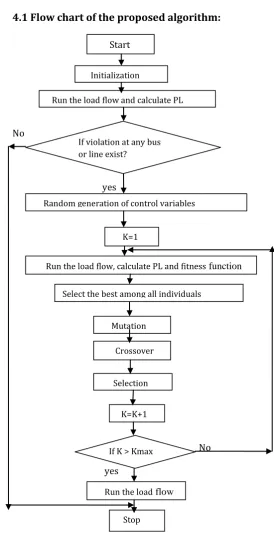
4.1 Flow chart of the proposed algorithm:
No
yes
No yes
Start
Initialization
Run the load flow and calculate PL
If violation at any bus or line exist?
Random generation of control variables
K=1
Run the load flow, calculate PL and fitness function
Select the best among all individuals
Mutation
Crossover
Selection
K=K+1
If K > Kmax
Stop
© 2015, IRJET.NET- All Rights Reserved
Page 1858
4.2 DE algorithm:
The DE algorithm is given below:
Step1: Generate an initial population randomly within the control variable bounds.
Step2: For each individual in the population, run power flow algorithm such as Newton Raphson method, to find the operating points.
Step3: Evaluate the fitness of the individuals according to Equations
Step4: Perform differentiation (mutation) and crossover as described in above Sections to create offspring from parents.
Step5: Perform Selection as described in above Section between parent and offspring. While using the penalty parameter-less method of constraint handling the following criteria are enforced while selecting the individuals for the next generation.
Any feasible solution is preferred to any infeasible solution.
Among two feasible solutions, the one having better objective function value is preferred.
Among two infeasible solutions, the one having smaller constraint violation is preferred.
Step6: Store the best individual of the current generation. Step7: Repeat steps 2 to 6 till the termination criteria is met (maximum number of generations).
4.3 Case Study:
To prove the effectiveness of the proposed algorithm, it has been tested on two standard IEEE test systems. Results obtained by simulation using differential evolutionary algorithm done in MATLAB, are provided in this section. Simulation is carried out on IEEE 14 and IEEE 30bus test systems.
Case 1: IEEE-14
bus test system:
The single line diagram of an IEEE 14-bus test system is shown below:
Fig-4.3.1:
Network diagram of IEEE 14-bus test systemThis system has 8-control variables as follows:
5-generators bus voltage magnitudes and 3-tap settings of transformers. Table2 shows the optimal setting of the control variables of 14-bus system.
Table 2:
optimal setting of the control variables of 14-bussystem: Serial Number
Control Variable
Initial Value Final Value ( DEA)
1 V1 1.0600 1.0425
2 V2 1.0450 1.0309
3 V3 1.0100 0.9956
4 V4 1.0700 0.9969
5 V5 1.0900 1.0179
6 T1 0.9320 0.9512
7 T2 0.9780 0.9855
8 T3 0.9690 0.9782
Power loss in MW 13.89 12.57 Voltage Deviation Index 0.9962 0.0446
Fig: 4.3.2 shows the convergence characteristics of 14 bus test system obtained by using the proposed algorithm:
© 2015, IRJET.NET- All Rights Reserved
Page 1859
Fig: 4.3.3 shows the voltage profile of 14 bus test systemobtained by using the proposed algorithm.
Fig: 4.3.3:
voltage profile of 14 bus test systemTable3:
comparison of results with different methods:PSO[9] IPM[10] Proposed Algorithm 13.327 MW 13.246 MW 12.57 MW
From the initial value of 13.89 MW the power loss is reduced to 12.57 MW. In order to evaluate the performance of differential evolutionary computation, the results were compared with popular Particle Swarm Optimization (PSO) and conventional Interior Point Method (IPM).
The proposed algorithm is also capable of reducing the total voltage deviation from an initial value of 0.9962 to 0.0446.
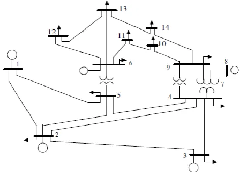
Case2: IEEE-30
bus test system:
The single line diagram of an IEEE 30-bus test system is shown below:
Fig-4.3.4:
Network diagram of IEEE 30-bus test systemThis system has 10-control variables as follows:
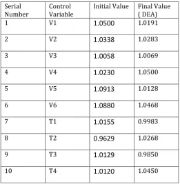
6-generators bus voltage magnitudes and 4-tap settings of transformers. Table: 4 Shows the optimal setting of the control variables of 30-bus system:
Table 4:
optimal setting of the control variables of 30-bussystem: Serial Number
Control Variable
Initial Value Final Value ( DEA)
1 V1
1.0500
1.01912 V2
1.0338
1.02833 V3
1.0058
1.00694 V4
1.0230
1.05005 V5
1.0913
1.01286 V6
1.0880
1.04687 T1
1.0155
0.99838 T2
0.9629
1.02689 T3
1.0129
0.9850© 2015, IRJET.NET- All Rights Reserved
Page 1860
Power loss in MW 5.822 4.720Voltage Deviation Index 1.9035 0.3079
Fig: 4.3.5 shows the convergence characteristics of 30 bus test system obtained by using the proposed algorithm.
Fig: 4.3.5:
convergence characteristics of 30 bus systemFig: 4.3.6 shows the voltage profile of 30 bus test system obtained by using the proposed algorithm.
Fig: 4.3.6:
voltage profile of 30 bus test systemTable5:
comparison of results with different methods:
SGA[12] PSO[11] Proposed Algorithm 4.98 MW 4.9262 MW 4.720 MW
From the initial value of 5.822 MW the power loss is reduced to 4.720 MW. In order to evaluate the performance of differential evolutionary computation, the
results were compared with popular Particle Swarm Optimization (PSO) and standard genetic algorithm (SGA). The proposed algorithm is also capable of reducing the total voltage deviation from an initial value of 1.9035 to 0.3079.
For both the cases, the DE population size is taken equal to 30. The maximum number of generations is 500, Mutation factor is F=0.6, and crossover rate is RC=0.8. The penalty factors in equation (2.5) are chosen as the multiples of 100. For both the cases, 20 runs have been performed for the objective function and the results which follow are the best solution of these 20 runs.
5. CONCLUSIONS
In this paper, an efficient DE solution to the ORPD problem has been presented for determination of the global or near-global optimum solution for optimal reactive power dispatch and voltage deviation in PQ buses. The main advantages of this DE to the ORPD problem are optimization of different type of objective function, real coded of both continuous and discrete control variables, and easily handling nonlinear constraints. The proposed algorithm has been tested on two IEEE bus systems i.e.IEEE-14 bus and IEEE-30 bus systems, to minimize the active power loss. The optimal setting of control variables are obtained in both continuous and discrete value. The results were compared with the other heuristic methods such as SGA. IPM and PSO algorithm reported in the literature and demonstrated its effectiveness and robustness.
ACKNOWLEDGEMENT
Through this paper, I would like to thank the authors of various research articles and books that I referred to.
REFERENCES
[1] K.Y. Lee, Y.M. Park, J.L. Ortiz, A united approach to optimal real and reactive power dispatch, IEEE Trans. Power Appar. Syst PAS, 104 (5) (1985) 1147-1153.
[2] S. Granville, Optimal reactive power dispatch through
interior point methods, IEEE Trans. Power Syst. 9 (1) (1994) 98–105.
[3] K. Iba, Reactive power optimization by genetic algorithms, IEEE Trans. Power Syst. 9 (2) (1994) 685–692.
[4] Q.H. Wu, J.T. Ma, Power system optimal reactive power dispatch using evolutionary programming, IEEE Trans Power. Syst. 10 (3) (1995) 1243–1249.
© 2015, IRJET.NET- All Rights Reserved
Page 1861
[6] R. Storn, K. Price, Differential Evolution—A Simpleand Efficient Adaptive Scheme for Global Optimization over Continuous Spaces, Technical Report TR-95-012, ICSI, 1995.
[7] D. Karaboga, S. Okdem, A simple and global optimization algorithm for engineering problems: differential evolution algorithm, Turk. J. Electr. Eng. 12 (1)(2004).
[8] Z. Daniela, A comparative analysis of crossover variants in differential evolution, Comput. Sci. Inform. Technol. (2007) 171–181.
[9] Yoshida H, Fukuyama Y, Kawata K, Takayama S, Nakanishi Y. A particle swarm optimization for reactive power and voltage control considering voltage security assessment. IEEE Trans Power Syst 2001;15(4):1232–9.
[10]Torres GL, Quintana VH. An interior-point method for nonlinear optimal power flow using rectangular coordinates. IEEE Trans Power Syst 1998;13(4):1211–8.
[11]B. Zhao, C. X. Guo, and Y.J. CAO. Multiagent-based particle swarm optimization approach for optimal reactive power dispatch. IEEE Trans. Power Syst. Vol. 20, no. 2, pp. 1070-1078, May 2005.
[12]Q.H. Wu, Y.J.Cao, and J.Y. Wen. Optimal reactive power dispatch using an adaptive genetic algorithm. Int. J. Elect. Power Energy Syst. Vol 20. Pp. 563-569; Aug 1998.
BIOGRAPHIES
Bhaskar Mahanta is currently a P.G. Research scholar at Assam Engineering college, Assam.
Dr. Barnali Goswami is currently an