R E S E A R C H
Open Access
The shooting method and integral
boundary value problems of third-order
differential equation
Wenyu Xie and Huihui Pang
**Correspondence: [email protected] College of Science, China Agricultural University, Beijing, 100083, China
Abstract
In this paper, the existence of at least one positive solution for third-order differential equation boundary value problems with Riemann-Stieltjes integral boundary conditions is discussed. By applying the shooting method and the comparison principle, we obtain some new results which extend the known ones. Meanwhile, an example is worked out to demonstrate the main results.
Keywords: shooting method; positive solution; third-order; boundary conditions including Stieltjes integrals
1 Introduction
It is well known that third-order equations arise from many branches of applied mathe-matics and physics. For example, in the deflection of a curved beam having a constant or varying cross section, a three layer beam, electromagnetic waves or gravity driven flows []. There have been extensive studies on third-order differential equation BVPs (bound-ary value problems), for example [–]. Most of these results are obtained via applying the topological degree theory, the fixed point theorems on cones, the lower and upper so-lution method, the critical point theory and monotone technique. We refer the reader to [–] and the references therein.
Recently, the attention has shifted to BVPs with Stieltjes integral boundary condition since this kind of conditions has been considered a single framework of multipoint and integral type boundary conditions. For more comments on the Riemann-Stieltjes integral boundary condition and its importance, we refer the reader to [, ] and other related work such as [, ].
In the existing literature, there are very few papers dealing with third-order differential equations with Riemann-Stieltjes integral boundary conditions. We found that Graef and Webb [] studied the following problem:
u(t) =g(t)f(t,u(t)), t∈(, ),
u() =α[u], u(p) = , u() +β[u] =λ[u],
wherep>, andα[u],β[u], andλ[v] are linear functional onC[, ] given by a Riemann-Stieltjes integral. The existence of multiple positive solutions is obtained by the application of the fixed point index theory.
In , Jankowski [] used a fixed point theorem to establish the existence of at least three non-negative solutions of some nonlocal BVPs to the third-order differential equa-tion
⎧ ⎪ ⎨ ⎪ ⎩
x(t) +h(t)f(t,x(α(t))) = , t∈(, ),
x() =x() = ,
x() =βx(η) +λ[x], β> ,η∈(, ),
whereλdenotes a linear functional onC(J) given byλ[x] =x(t)d(t) involving a Stielt-jes integral with a suitable functionof bounded variation.
In [], the author applied the method of lower and upper solutions to generate an itera-tive technique and discussed the existence of solutions of nonlinear third-order ordinary differential equations with integral boundary conditions. Pang and Xie [] investigated the existence of concave positive solutions and established corresponding iterative schemes for a third-order differential equation with Riemann-Stieltjes integral boundary conditions using the monotone iterative technique.
It is well known that the classical shooting method could be effectively used to establish the existence and multiplicity results for differential equation BVPs. To some extent, this approach has an advantage over the traditional methods. Readers can see [–] and the references therein for details.
Using the shooting method, Henderson [] obtained solutions of the three point BVP for the second-order equation
y=fx,y,y , y(x) =y, y(x) –y(x) =y,
wheref : (a,b)×R→Ris continuous,a<x
<x<x<b, andy,y∈R.
In [], by applying the shooting method and the comparison principle, Wang investi-gated the existence results of positive solutions for the Riemann-Stieltjes integrals BVPs
u(t) +a(t)f(u(t)) = , <t< ,
u() = , u() =αηu(s)ds,
wheref ∈C([,∞); [,∞)) and <η< ,α≥ are given constants, <αη< .
However, to the best of our knowledge, no paper has considered the existence of positive solutions for third-order differential equation with the shooting method till now. Moti-vated by the excellent work mentioned above, in this paper, we try to employ the shooting method to establish the criteria for the existence of positive solutions to the following third-order differential equation with integral boundary condition:
u(t) +h(t)f(u(t),u(t)) = , <t< ,
where α[u] =u(s)dA(s), β[u] =u(s)dB(s), andα[u], β[u] are linear functions on
C[, ] given by the Riemann-Stieltjes integral, A(t), B(t) are suitable functions of a bounded variation.
Set
fx=lim
v→xsup maxu∈[,+∞)
f(u,v)
v , fx=vlim→xinf minu∈[,+∞)
f(u,v)
v .
In this paper, we always assume
(H) f ∈C([,∞)×[,∞); [,∞)),f(u,v)≡;
(H) h∈C([, ]; [,∞));
(H)
dA(t) > , <
dB(t) < .
2 Preliminaries
Define an operatorA:C[, ]→C[, ] as
Ay(t) =
G(t,s)y(s)ds (.)
fort∈[, ], where
G(t,s) = –dB(t)
s
dB(t), ≤s≤t≤,
–s dB(t), ≤t≤s≤,
is the Green function for the following first-order differential equation:
u(t) =y(t), <t< ,
u() =β[u].
Lety=u, then BVP (.) is equivalent to the following second-order BVP:
y(t) +h(t)f(Ay(t),y(t)) = , <t< ,
y() =α[y], y() = . (.)
Lemma . If y is a positive solution of(.),then u is a positive solution of(.).
Proof Assumeyis a positive solution of (.), theny(t) > fort∈(, ) and it follows from
u(t) =Ay(t) thatu(t) satisfies (.). Assume on the contrary that there is at∈(, ) such
thatu(t) =mint∈(,)u(t)≤, thenu(t) = andu(t)≥, which yieldsy(t) =u(t) = .
This contradicts the assumption thatyis a positive solution of (.). Hence,u(t) > for all
t∈(, ).
The principle of the shooting method converts the BVP into an IVP (initial value prob-lem) by finding suitable initial valuesmsuch that equation (.) comes with the initial value condition as
y(t) +h(t)f(Ay(t),y(t)) = , <t< ,
Under the assumptions (H)-(H), denote byy(t,m) the solution of the IVP (.). We
assume thatf is strong continuous enough to guarantee thaty(t,m) is uniquely defined and that it depends continuously on bothtandm. The discussion of this problem can be found in []. Therefore the solution of IVP (.) exists.
Denote
k(m) = y(,m)
y(t,m)dA(t)
, ϕ(m) =y(,m) –
y(t,m)dA(t).
Then solving (.) is equivalent to finding am∗such thatk(m∗) = orϕ(m∗) = .
Lemma .(Sturm comparison theorem) [] Letϕandϕbe non-trivial solutions of
the equations
y+q(x)y= , y+q(x)y= ,
respectively,on an interval I;here qand qare continuous functions such that q(x)≤q(x)
on I.Then between any two consecutive zeros xand xofϕ,there exists at least one zero
ofϕunless q(x)≡q(x)on(x,x).
Lemma . Let y(t,m),z(t,m),Z(t,m)be the solution of the IVPs,respectively,
y(t) +F(t)y(t) = , y() =m, y() = ,
z(t) +g(t)z(t) = , z() =m, z() = ,
Z(t) +G(t)Z(t) = , Z() =m, Z() = ,
and suppose that F(t),g(t),and G(t)are continuous functions defined on[, ]such that g(t)≤F(t)≤G(t), t∈[, ].
If Z(t,m)does not vanish in(, ],then for any≤ξ≤s≤,we have z(ξ,m)
z(s,m) ≤
y(ξ,m)
y(s,m) ≤
Z(ξ,m)
Z(s,m), (.)
and hence,for any≤s≤,we have z(,m)
z(s,m)dA(s)
≤ y(,m) y(s,m)dA(s)
≤ Z(,m) Z(s,m)dA(s)
. (.)
Proof The proof for (.) can be found in []. The continuity of the integrands implies the existence of the Riemann integral. In view of the definition of Stieltjes integral, by using
the inequality of the limit, we have (.).
Lemma . Assume that(H)-(H)hold and <
dA(t) < ,then BVP(.)has no
pos-itive solution.
z(t) =mof
z(t) + z(t) = , z() =m, z() = .
By Lemma ., we have
y(,m)
y(s,m)dA(s)
≥ z() z(s)dA(s)
= m
mdA(s)=
dA(s)
.
In fact,y(,m) =y(s,m)dA(s). That is,dA(s)≥.
Hence, we needdA(s)≥, and we assumedA(s) > in (H) in order to satisfy
(.).
3 Main results
In the following, we assume thatA(t) has continuous derivative functionα(t) andα(t) > fort∈[, ] such thatdA(t) =α(t)dt> .
For the sake of convenience, we denote
max
≤t≤
h(t)=hL, min
≤t≤
h(t)=hl,
max
≤t≤
α(t)=αL, min
≤t≤
α(t)=αl.
It is obvious thatαL≥αl> .
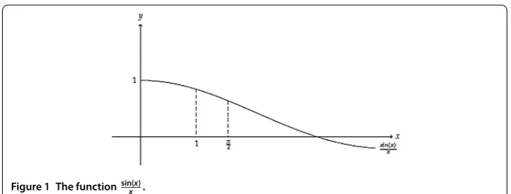
Lemma . Assume that(H)-(H)hold.Then there exist a solution x=A∈(,π)such
that
g(x) :=
αlsinx
x ≥ (.)
and a solution x=A∈(,π)such that
g(x) :=
αLsinx
x ≤. (.)
Proof From (H) and the Figure , we can easily get Lemma ..
Theorem . Assume that(H)-(H)hold.Suppose one of the following conditions holds:
Then problem(.)has at least one positive solution,where A=min{A,A}, A¯=max{A,A},
and A,Aare defined in(.)and(.),respectively.
Proof As we mentioned above, BVP (.) having a positive solution is equivalent to BVP (.) having a positive solution.
(i) Since ≤f<A
hL, there exists a positive numberrsuch that
f(Ay,y)
On the other hand, the second inequality in (i) implies that there exists a numberLlarge enough such that
and there exists a positive number<Asmall enough that
f(Ay,y)
y >
(A+)
hl , y≥L. (.)
Next, we will find a positive numberm∗such thatϕ(m∗)≥. There exist a valuem∗and a positive numberσsuch that
< A
A+ ≤
Since the solutiony(t,m) is concave andy(,m) = , it hits the liney=Lat most one time for the constantLdefined in (.) andt∈(, ]. We denote the intersecting time by
¯
δmprovided it exists. Henceforth, denoteIm= (,δ¯m]⊆(, ]. Ify(,m)≥L, thenδ¯m= .
The discussion is divided into three steps.
Step. We claim that there exists a valuemlarge enough such that ≤y(t,m)≤Lfor
t∈[δ¯m, ] andy(t,m)≥Lfort∈Im.
Otherwise, providedy(t,m)≤Lfor allt∈[, ] asm→ ∞, then by integrating both sides of equation (.) from tot, we have
y(t,m) =m–
t
(t–s)h(s)fAy(s,m),y(s,m) ds. (.)
Hence, from (.) and the continuity off(Ay,y), we have
m=y(,m) +
( –s)h(s)fAy(s,m),y(s,m) ds≤L+LfhL. (.)
SinceAis defined in (.) as a continuous operator that depends ony, forf(Ay,y) there exists a maximum fory∈[,L]. DenoteLf =maxy∈[,L]f(Ay,y). If we choosem>L+LfhL,
(.) will lead to a contradiction.
Sincey(t,m) is continuous and concave, there exists a numbermlarge enough such
thaty(t,m)≥Lfort∈Im.
Step. There exists a monotonically increasing sequence{mk}such that the sequence
¯
δmk is increasing onmk. That is,
Im⊂Im⊂ · · · ⊂Imk· · · ⊆(, ] andy(t,mk)≥Lfort∈Imk.
We prove that
¯
δmk–<δ¯mk, k= , , . . . formk–<mk. (.) Sincef guarantees thaty(t,m) is uniquely defined, the solutiony(t,mk–) andy(t,mk) have
no intersection in the interval [δ¯mk–, ). It follows from
y(,mk) =mk>mk–=y(,mk–)
that
y(δ¯mk–,mk) >y(δ¯mk–,mk–). Thus we have (.).
Whenk= , see the relationship ofmandImin Figure .
Step. Seek a valuem∗and a positive numberσsuch that < A
A+ ≤σ≤ andy(t,m
∗
)≥
Lfort∈(,σ].
Following step , step , and the extension principle of solutions, there exists a positive integernlarge enough such that
¯ δmn≥
A
A+
Figure 2 The relationship ofmandIm.
If we takenm∗=mn,σ=δ¯mn, then
σ(A+)≥A. (.)
In the following, we prove thatk(m∗)≥ for the selectedm∗andσ.
Setz(t) =m∗cosσ(A+)t, thenz(t) satisfies the following IVP:
z(t) +σ(A+)z(t) = , z() =m∗, z() = , (.)
whereσ≤. From (.), we have
f(Ay,y)
y >
σ(A +)
hl , y≥L.
Further, noting that y(,m∗) >L (this time σ = ) or y(,m∗)≤y(σ,m∗) =L, then by
Lemma . and Lemma . we have
km∗ = y(,m ∗
)
y(t,m∗)dA(t)
≥ z(,m∗)
z(t,m∗)dA(t)
=
cos[σ(A+)t]dA(t)
≥
αL
cos[σ(A+)t]dt
= σ(A+)
αLsin[σ(A
+)]≥
A
αLsinA
≥
, (.)
which impliesϕ(m∗)≥.
From (.) and (.), we can find am∗ betweenm∗ andm∗ such thaty(t,m∗) is the solution of (.). So thatu(t,m∗) =Ay(t,m∗) is the solution of (.).
Now, we prove for (ii).
Setz(t) =m∗cosσ(A+)tandZ(t) =m∗cos(At) fort∈[, ], thenz(t) andZ(t) satisfy
the following IVPs, respectively:
z(t) +σ(A+)z(t) = , z() =m∗, z() = , (.)
Similar to (.) and (.), it follows from (.) and (.)-(.) that
least one positive solutionu(t).
Competing interests
The authors declare that there is no conflict of interests regarding the publication of this paper.
Authors’ contributions
The authors declare that the study was realized in collaboration with the same responsibility. All authors read and approved the final manuscript.
Acknowledgements
The work is supported by Chinese Universities Scientific Fund (Project No.2016LX002)
References
1. Gregus, M: Third Order Linear Differential Equations. Mathematics and Its Applications. Reidel, Dordrecht (1987) 2. Zhou, C, Ma, D: Existence and iteration of positive solutions for a generalized right-focal boundary value problem
withp-Laplacian operator. J. Math. Anal. Appl.324, 409-424 (2006)
3. Webb, JRL, Infante, G: Positive solutions of nonlocal boundary value problems: a unified approach. J. Lond. Math. Soc.
74, 673-693 (2006)
4. Webb, JRL, Infante, G: Nonlocal boundary value problems of arbitrary order. J. Lond. Math. Soc. (2)79, 238-258 (2009) 5. Webb, JRL: Positive solutions of some higher order nonlocal boundary value problems. Electron. J. Qual. Theory
Differ. Equ.2009, 29 (2009)
6. Graef, JR, Webb, JRL: Third order boundary value problems with nonlocal boundary conditions. Nonlinear Anal.71, 1542-1551 (2009)
7. Jankowski, T: Existence of positive solutions to third order differential equations with advanced arguments and nonlocal boundary conditions. Nonlinear Anal.75, 913-923 (2012)
8. Boucherif, A, Bouguima, SM, Benbouziane, Z, Al-Malki, N: Third order problems with nonlocal conditions of integral type. Bound. Value Probl.2014, 137 (2014)
9. Pang, H, Xie, W, Cao, L: Successive iteration and positive solutions for a third-order boundary value problem involving integral conditions. Bound. Value Probl.2015, 139 (2015)
10. Sun, Y: Positive solutions of singular third-order three-point boundary value problem. J. Math. Anal. Appl.306, 589-603 (2005)
11. Lin, X, Du, Z, Liu, W: Uniqueness and existence results for a third-order nonlinear multi-point boundary value problem. Appl. Math. Comput.205, 187-196 (2008)
12. El-Shahed, M: Positive solutions for nonlinear singular third order boundary value problem. Commun. Nonlinear Sci. Numer. Simul.14, 424-429 (2009)
13. Graef, JR, Kong, L: Positive solutions for third order semipositone boundary value problems. Appl. Math. Lett.22, 1154-1160 (2009)
14. Li, S: Positive solutions of nonlinear singular third-order two-point boundary value problem. J. Math. Anal. Appl.323, 413-425 (2006)
15. Liu, Z, Ume, JS, Kang, SM: Positive solutions of a singular nonlinear third order two-point boundary value problems. J. Math. Anal. Appl.326, 589-601 (2007)
16. Yao, Q: The existence and multiplicity of positive solutions for a third-order three-point boundary value problem. Acta Math. Appl. Sin.19, 117-122 (2003)
17. Yao, Q, Feng, Y: The existence of solution for a third-order two-point boundary value problem. Appl. Math. Lett.15, 227-232 (2002)
18. Kwong, MK: The shooting method and multiple solutions of two/multi-point BVPs of second-order ODE. Electron. J. Qual. Theory Differ. Equ.2006, 6 (2006)
19. Hopkins, B, Kosmatov, N: Third-order boundary value problems with sign-changing solutions. Nonlinear Anal.67, 126-137 (2007)
20. Iturriage, L, Sanchez, J: Exact number of solutions of stationary reaction-diffusion equations. Appl. Math. Comput.
216, 1250-1258 (2010)
21. Kwong, MK, Wong, JSW: The shooting method and nonhomogeneous multipoint BVPs of second-order ODE. Bound. Value Probl.2007, 64012 (2007)
22. Agarwal, RP: The numerical solution of multipoint boundary value problems. J. Comput. Appl. Math.5, 17-24 (1979) 23. Henderson, J: Uniqueness implies existence for three-point boundary value problems for second order differential
equations. Appl. Math. Lett.18, 905-909 (2005)
24. Wang, H, Ouyang, Z, Tang, H: A note on the shooting method and its applications in the Stieltjes integral boundary value problems. Bound. Value Probl.2015, 102 (2015)