R E S E A R C H
Open Access
Dynamics of a two-dimensional system of
rational difference equations of Leslie
–
Gower
type
S Kalabu
š
i
ć
1, MRS Kulenovi
ć
2*and E Pilav
1* Correspondence: [email protected] 2Department of Mathematics, University of Rhode Island, Kingston, RI 02881-0816, USA Full list of author information is available at the end of the article
Abstract
We investigate global dynamics of the following systems of difference equations ⎧
⎪ ⎨ ⎪ ⎩
xn+1= α1 +β1xn A1+yn yn+1= γ2
yn A2+B2xn+yn
, n= 0, 1, 2,. . .
where the parametersa1, b1, A1,g2,A2,B2 are positive numbers, and the initial
conditionsx0 andy0 are arbitrary nonnegative numbers. We show that this system
has rich dynamics which depends on the region of parametric space. We show that the basins of attractions of different locally asymptotically stable equilibrium points or non-hyperbolic equilibrium points are separated by the global stable manifolds of either saddle points or non-hyperbolic equilibrium points. We give examples of a globally attractive non-hyperbolic equilibrium point and a semi-stable non-hyperbolic equilibrium point. We also give an example of two local attractors with precisely determined basins of attraction. Finally, in some regions of parameters, we give an explicit formula for the global stable manifold.
Mathematics Subject Classification (2000)
Primary: 39A10, 39A11 Secondary: 37E99, 37D10
Keywords:Basin of attraction, Competitive map, Global stable manifold, Monotoni-city, Period-two solution
1 Introduction
In this paper, we study the global dynamics of the following rational system of differ-ence equations
⎧ ⎪ ⎨ ⎪ ⎩
xn+1= α1 +β1xn A1+yn yn+1= γ2
yn A2+B2xn+yn
, n= 0, 1, 2,. . . (1)
where the parametersa1, b1, A1, g2,A2, B2 are positive numbers and initial
condi-tionsx0andy0are arbitrary nonnegative numbers.
System (1) was mentioned in [1] as one of three systems of Open Problem 3, which asked for a description of the global dynamics of some rational systems of difference equations. In notation used to label systems of linear fractional difference equations
used in [1], System (1) is referred to as (29, 38). This system is dual to the system where the roles of xnandynare interchanged, which is labeled as (29, 38) in [1], and so all results proven here extend to the latter system. In this paper, we provide a pre-cise description of the global dynamics of the System (1). We show that System (1) may have between zero and three equilibrium points, which may have different local character. If System (1) has one equilibrium point, then this point is either locally asymptotically stable or saddle point or non-hyperbolic equilibrium point. If System (1) has two equilibrium points, then they are either locally asymptotically stable and non-hyperbolic, or locally asymptotically stable and saddle point. If System (1) has three equilibrium points, then two of equilibrium points are locally asymptotically stable and the third point, which is between these two points in southeast ordering defined below, is a saddle point. The major problem for global dynamics of the System (1) is determining the basins of attraction of different equilibrium points. The difficulty in analyzing the behavior of all solutions of the System (1) lies in the fact that there are many regions of parameters where this system possesses different equilibrium points with different local character and that in several cases, the equilibrium point is non-hyperbolic. However, all these cases can be handled by using recent results from [2].
System (1) is a competitive system, and our results are based on recent results about competitive systems in the plane, see [2,3]. System (1) can be used as a mathematical model for competition in population dynamics. In fact, second equation in (1) is of Leslie-Gower type, and first equation can be considered to be of Leslie-Gower type with stocking which is represented with the terma1, see [4-6].
In the next section, we present some general results about competitive systems in the plane. Section 3 contains some basic facts such as the non-existence of period-two solution of System (1). Section 4 analyzes local stability which is fairly complicated for this system. Finally, Section 5 gives global dynamics for all values of parameters.
2 Preliminaries
A first-order system of difference equations
xn+1=f(xn,yn)
yn+1=g(xn,yn) , n= 0, 1, 2,. . . (2)
where S ⊂ℝ2, (f, g):S ®S,f, gare continuous functions is competitiveif f(x, y) is non-decreasing in xand non-increasing in y, and g(x, y) is non-increasing in xand non-decreasing in y. If bothfand gare non-decreasing in x andy, the System (2) is
cooperative. Competitive and cooperative maps are defined similarly.Strongly competi-tivesystems of difference equations or strongly competitive maps are those for which the functionsfandgare coordinate-wise strictly monotone.
dimensional systems. Part of the reason for this situation is de Mottoni and Schiaffino theorem given below, which provides relatively simple scenarios for possible behavior of many two-dimensional discrete competitive and cooperative systems. However, this does not mean that one cannot encounter chaos in such systems as has been shown by Smith, see [17].
If v = (u, v)Î ℝ2, we denote withQl (v), ℓ Î {1, 2, 3, 4}, the four quadrants inℝ2
relative to v, i.e.,Q1 (v) = {(x,y)ℝ2: x≥u,y ≥v},Q2 (v) = {(x,y)Îℝ2:x ≤u, y≥ v},
and so on. Define the South-Eastpartial order ≼seonℝ2 by (x, y)≼se(s, t) if and only if x≤s andy ≥t. Similarly, we define the North-Eastpartial order≼neonℝ2by (x, y)
≼ne (s, t) if and only if x ≤s and y ≤ t. ForA⊂ ℝ2 and x Î ℝ2, define thedistance
fromx toAas dist(x,A) = inf{||x-y||: yÎA}. By intA, we denote the interior of a set A.
It is easy to show that a mapFis competitive if it is non-decreasing with respect to the South-East partial order, that is, if the following holds:
x1 y1
se
x2 y2
⇒F
x1 y1
seF
x2 y2
. (3)
For standard definitions of attracting fixed point, saddle point, stable manifold, and related notions see [11].
We now state three results for competitive maps in the plane. The following defini-tion is from [17].
Definition 1LetS be a nonempty subset ofℝ2.A competitive map T:S ®Sis said to satisfy condition (O+) if for every x, y inS, T(x)≼neT (y)implies x≼ney, and T is
said to satisfy condition(O-)if for every x, y inS, T(x)≼neT(y)implies y≼nex. The following theorem was proved by de Mottoni and Schiaffino [20] for the Poin-caré map of a periodic competitive Lotka-Volterra system of differential equations. Smith [14,15] generalized the proof to competitive and cooperative maps.
Theorem 1LetS be a nonempty subset ofℝ2. If T is a competitive map for which(O
+) holds then for all xÎS, {Tn(x)}is eventually componentwise monotone. If the orbit of x has compact closure, then it converges to a fixed point of T. If instead (O-)holds, then for all x ÎS, {T2n(x)} is eventually componentwise monotone. If the orbit of x has compact closure in S, then its omega limit set is either a period-two orbit or a fixed point.
The following result is from [17], with the domain of the map specialized to be the cartesian product of intervals of real numbers. It gives a sufficient condition for condi-tions (O+) and (O-).
Theorem 2 Letℛ ⊂ℝ2 be the cartesian product of two intervals inℝ. Let T:ℛ ® ℛ be a C1 competitive map. If T is injective and detJT (x)>0 for all xÎ ℛ then T
satisfies (O+). If T is injective anddetJT(x)<0for all xÎℛ then T satisfies(O-). The following result is a direct consequence of the Trichotomy Theorem of Dancer and Hess, see [3] and [21] and is helpful for determining the basins of attraction of the equilibrium points.
Next result is well-known global attractivity result that holds in partially ordered Banach spaces as well, see [21].
Theorem 3 Let T be a monotone map on a closed and bounded rectangular regionℛ ⊂ℝ2
. Suppose that T has a unique fixed pointe¯ inℛ. Thene¯ is a global attractor of T onℛ.
The following theorems were proved by Kulenović and Merino [2] for competitive systems in the plane, when one of the eigenvalues of the linearized system at an equili-brium (hyperbolic or non-hyperbolic) is by absolute value smaller than 1 while the other has an arbitrary value. These results are useful for determining basins of attrac-tion of fixed points of competitive maps.
Theorem 4Let T be a competitive map on a rectangular region ℛ⊂ℝ2. Let x∈R
be a fixed point of T such thatΔ: =ℛ ∩int(Q1(x)∪Q3(x))is nonempty (i.e., xis not the NW or SE vertex ofℛ), and T is strongly competitive onΔ. Suppose that the follow-ing statements are true.
a.The map T has a C1extension to a neighborhood ofx.
b.The Jacobian JT(x)of T atxhas real eigenvaluesl, μsuch that0 <|l| <μ, where |l|<1, and the eigenspace Elassociated withlis not a coordinate axis.
Then there exists a curveC⊂ℛthrough xthat is invariant and a subset of the basin of attraction of x, such thatCis tangential to the eigenspace Elat x, andCis the graph of a strictly increasing continuous function of the first coordinate on an interval. Any endpoints of Cin the interior of ℛare either fixed points or minimal period-two points. In the latter case, the set of endpoints ofCis a minimal period-two orbit of T.
The situation where the endpoints ofCare boundary points of ℛ is of interest. The following result gives a sufficient condition for this case.
Theorem 5 For the curve Cof Theorem 4 to have endpoints in∂ℛ, it is sufficient that at least one of the following conditions is satisfied.
i.The map T has no fixed points nor periodic points of minimal period-two inΔ. ii.The map T has no fixed points inΔ, det JT(x)>0, andT(x) = xhas no solutions xÎΔ.
iii. The map T has no points of minimal period-two in Δ, det JT(x)<0, and T(x) = xhas no solutions xÎΔ.
The next result is useful for determining basins of attraction of fixed points of com-petitive maps.
Theorem 6 (A) Assume the hypotheses of Theorem4, and letCbe the curve whose existence is guaranteed by Theorem 4. If the endpoints ofCbelong to∂ℛ, thenC sepa-rates ℛinto two connected components, namely
W−:={x∈R\C:∃y∈Cwithxsey} and W+:={x∈R\C:∃y∈Cwithysex}, (4)
such that the following statements are true.
(i)W-is invariant, anddist (Tn(x), Q2(x))¯ →0as n→ ∞for everyx∈W .
(B) If, in addition to the hypotheses of part(A),x is an interior point ofℛand T is C2 and strongly competitive in a neighborhood of x, then T has no periodic points in the boundary of(Q1(x)∪Q3(x))except forx, and the following statements are true.
(iii)For everyxÎW-there exists n0ÎN such that Tn(x)ÎintQ2(x)for n≥n0.
(iv)For everyxÎW+there exists n0 ÎNsuch that Tn(x)ÎintQ4(x)for n≥n0.
IfTis a map on a setℛand ifxis a fixed point ofT, thestable setWs(x)ofxis the set{x∈R:Tn(x)→x}andunstable setWu(x)ofxis the set
{x∈R: there exists{xn}0n=−∞⊂Rs.t.T(xn) = xn+1, x0= x, and lim
n→−∞xn= x}
WhenTis non-invertible, the setWs(x)may not be connected and made up of infi-nitely many curves, or Wu(x)may not be a manifold. The following result gives a description of the stable and unstable sets of a saddle point of a competitive map. If the map is a diffeomorphism on ℛ, the sets Ws(x)andWu(x)are the stable and unstable manifolds of x.
Theorem 7In addition to the hypotheses of part(B)of Theorem6, suppose thatμ>1
and that the eigenspace Eμassociated withμis not a coordinate axis. If the curveCof Theorem4 has endpoints in∂ℛ, thenCis the stable setWs(x)ofx, and the unstable set Wu(x)of x¯ is a curve inℛ that is tangential to Eμ at xand such that it is the graph of a strictly decreasing function of the first coordinate on an interval. Any end-points ofWu(x)inℛ are fixed points of T.
The following result gives information on localdynamics near a fixed point of a map when there exists a characteristic vector whose coordinates have negative product and such that the associated eigenvalue is hyperbolic. This is a well-known result, valid in much more general setting that we include it here for completeness. A point (x, y) is a
subsolution ifT(x, y)≼se (x, y), and (x, y) is a supersolution if (x, y)≼se T(x, y). An
order interval 〚(a, b), (c, d)〛is the cartesian product of the two compact intervals [a, c] and [b, d].
Theorem 8 Let T be a competitive map on a rectangular set ℛ⊂ ℝ2 with an iso-lated fixed point x∈Rsuch thatR∩int (Q2(x)¯ ∪Q4(x))¯ =∅. Suppose T has a C1
extension to a neighborhood ofx. Letv = (v(1), v(2))Îℝ2 be an eigenvector of the Jaco-bian of T at x, with associated eigenvalue μ Î ℝ. Ifv(1)v(2) < 0, then there exists an order intervalℐwhich is also a relative neighborhood of xsuch that for every relative neighborhood U ⊂ℐofxthe following statements are true.
i. Ifμ > 1,then U∩intQ2(x)contains a subsolution and U∩intQ4(x)contains a supersolution. In this case for everyx ∈I∩int (Q2(x)∪Q4(x))there exists N such that Tn(x)∉ℐfor n≥N.
ii.Ifμ< 1, then U∩intQ2(x)contains a supersolution andU∩intQ4(x)contains
a subsolution. In this caseTn(x)→xfor everyxÎℐ.
3 Some basic facts
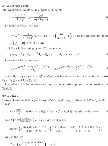
3.1 Equilibrium points
The equilibrium points (x,y) of System (1) satisfy¯
¯
x= α1+β1x¯ A1+y¯
, y¯= γ2y¯ A2+B2x¯+¯y
. (5)
Solutions of System (5) are:
(i)y¯= 0, x¯= α1
A1−β1, A1 >b1, i.e. E1=
α1 A1−β1
, 0
. Thus, the equilibrium point
E1= A1α−1β1, 0
exists ifA1>b1.
(ii) Ify¯= 0, then using System (5), we obtain
¯
y=γ2−A2−B2¯x, x¯2B2− ¯x(γ2+A1−A2−β1) +α1= 0. (6)
Solutions of System (6) are:
¯
x3,2= γ2
+A1−A2−β1±
√
D0 2B2
, y¯2,3= γ2−
A2−A1+β1±
√
D0
2 , (7)
where D0 = (g2 -A2 +A1 -b1)2 - 4B2a1 which gives a pair of the equilibrium points
E2= (x¯2,y¯2)andE3= (x¯3,y¯3).
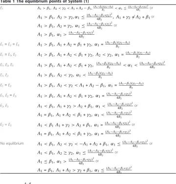
The criteria for the existence of the three equilibrium points are summarized in Table 1.
3.2 Injectivity
Lemma 1Assume that(x¯,y¯)is an equilibrium of the map T. Then the following holds:
1)If
B2>
A2β1
α1
, A1(B2α1−A2β1)γ2−(B2α1+ (A1−A2)β1)(A1A2−β1A2+B2α1) = 0, (8)
thenT x,A1A2β1+xA1B2β1
B2α1−A2β1
= (x¯,y¯)for all x≥0, where
(x¯,¯y) =
¯
x,A1A2β1+xA¯ 1B2β1 B2α1−A2β1
=
B2α1+A2β1 A1B2
,−A2β 2
1+A1A2β1+B2α1β1 B2α1−A2β1
.
That is the line
I=
x,A1A2β1+xA1B2β1 B2α1−A2β1
:x≥0
is invariant, equilibrium (x¯,¯y)∈Iand for (x, y) Î ℐ the following holds
T(x,y) = (x¯,y¯),that is every point of this line is mapped to the equilibrium point(x¯,¯y).
1.i)If(B2α1 − A2β1)2−A2
1B2α1>0then(¯x,y¯) =E3. 1.ii)If(B2α1 − A2β1)2−A2
1B2α1<0then(x¯,y¯) =E2. 1.iii)If(B2α1 − A2β1)2−A2
1B2α1= 0then(x¯,¯y) =E3=E2.
B2≤
Table 1 The equilibrium points of System (1)
Equation 11 implies
y= y¯α1+xy¯β1+xA1β1− ¯xA1β1
α1+¯xβ1 .
and Equation 12 is equivalent to
(x− ¯x)−¯yB2α1+¯yA2β1+A1A2β1+xA¯ 1B2β1 equilibrium of the mapT, then
B2>
which completes the proof of lemma.
3.3 Period-two solutions
In this section, we prove that System (1) has no minimal period-two solutions which will be essential for application of Theorem 4 and Corollary 6.
Lemma 2System(1)has no minimal period-two solution.
yy+A1
Put (18) into (15), we have that (15) is equivalent to
y+A1= 0 (19)
If (19) holds, then we obtain a negative solution. Now, assume that (20) holds. We have
Put (21) into (18), we obtain that (18) is equivalent to
−y2+(−A1−A2+β1+γ2)y−B2α1+β1(A2−γ2)+A1(γ2−A2)= 0 (22)
If (22) holds, we obtain the fixed points. So, we assume that (23) holds. Set
where
1:=(A1+β1) (A1−A2+β1−γ2) (B2α1+(A1−β1) (A2+γ2)).
Substituting this into (21), we have that the corresponding solutions are
x1= (2−
√
)
2B2(A1+β1) (A1(A1−A2+β1)+β1γ2)
x2= (2
+√)
2B2(A1+β1) (A1(A1−A2+β1)+β1γ2)
where
2:=(A1+β1)
−(A1+β1) γ22−
(A1+β1)2+B2α1
γ2+(−A1+A2−β1) (A2(A1+β1)−B2α1)
. (25)
□
Claim 1 AssumeΔ ≥0. Then we have:
a)If x1 ≥0then y1< 0. b)If x2≥0then y2< 0.
Proof. SinceT : [0, ∞)2 ® [0,∞)2,T(x1, y1) = (x2, y2) and T(x2, y2) = (x1,y1), it is obvious that if (xi, yi)Î [0,∞)2 holds thenT(xi, yi)Î [0,∞)2 fori= 1, 2. It is enough to show that the assumptions (x1,y1), (x2,y2)Î[0,∞)2 andT(x1, y1) = (x2,y2)≠(x1,
y1) lead to a contradiction.
Indeed, if A1(A1 - A2 +b1) +b1g2 > 0 then (x1, y1) ≺se (x2,y2). Since Tis strongly competitive map then (x2, y2) =T(x1, y1) <<seT(x2, y2) = (x1,y1) which is impossible since (x1,y1)≺se (x2,y2).
If A1(A1 -A2 +b1) +b1g2 < 0 then (x2, y2)≺se(x1, y1) Similarly, we have the same conclusion ifA1(A1-A2 +b1) +b1g2= 0. □
3.4 Boundedness of solutions
Lemma 3Assume that y0 = 0,x0Îℝ+. Then the following statements are true.
(i)If A1 >b1 thenyn= 0xn→ α
1
A1−β1,n®∞. (ii)If A1<b1 then yn= 0,xn®∞,n®∞.
(iii)If A1=b1,thenxn=x0+Aα11nand yn= 0,xn® ∞.
Assume that y0≠0 and(x0,y0)∈R+
2.Then the following statements are true.
(iv)xn+1≤Aα11 +βA11xnfor all n= 0, 1, 2,...
(v)yn≤g2,n≥N,yn+1≤C γA22
n
and
(a)xn→ A1α−1β1,A1 >b1.
(b)xn≤ A1α−1β1 +ε,ε> 0, A1 >b1.
(c)Ifg2 <A2 then yn® 0,n®∞
xn+1= α1
Lemma 3 follows from (27). □
4 Linearized stability analysis
The mapTassociated to System (1) is given by
T(x,y) =
The Jacobian matrix of the mapThas the form:
JT=
The determinant of (29) is given by
detJT(x¯,¯y) = β1
The characteristic equation has the form
λ2−λ
Theorem 9 Assume that A1>b1.Then there exists the equilibrium point E1 and:
The corresponding eigenvectors, respectively, are
v1= (1, 0), v2=
⎛
⎝ α1
A1(A1−β1) βα11− A1A2+(AB12−αβ11)−A2β1
, 1
⎞ ⎠.
(iii)E1is non-hyperbolic ifγ2−A2= AB12−αβ11.The eigenvalues areλ1= βA1
1, l2= 1. The
corresponding eigenvectors are − α1 (A1−β1)2, 1
and(1, 0).
Proof. Evaluating Jacobian (29) at the equilibrium pointE1(a1/(A1-b1), 0),
JT(E1) =
β1
A1 −
α1
A1(A1−β1) 0 (A1−β1)γ2
A2(A1−β1)+B2α1
. (30)
The determinant of (30) is given by
detJT(x¯,¯y) = β1γ2(
A1−β1) A1[A2(A1−β1) +B2α1]
.
The trace of (30) is
TrJT(x¯,¯y) = β1 A1
+ (A1−β1)γ2
A2(A1−β1) +B2α1 .
The characteristic equation associated to System (1) at E1has the form
β1
A1 −λ
(A1−β1)γ2
A2(A1−β1) +B2α1 −λ
= 0. (31)
From Equation 31 we have
λ1= β1
A1
, λ2= (A1−β1)γ2
A2(A1−β1) +B2α1 .
(i) IfA1>b1andγ2−A2< AB12−αβ11 thenl1 < 1 andl2< 1. Hence, E1is a sink.
(ii) IfA1>b1andγ2−A2> AB12−αβ11. Thenl1 < 1, andl2 < 1. Hence,E1is a saddle.
(iii) IfA1 >b1 andγ2−A2= AB12−αβ11. Then, using Equation 31, we have thatl1 < 1
andl2< 1.
From (30) we obtain the eigenvectors that correspond to these eigenvalues. □
We now perform a similar analysis for the other cases in table.
Theorem 10 Assume
A1> β1, A1+A2< β1+γ2, (
A1−β1) (γ2−A2)
B2 < α 1<(
A1−A2−β1+γ2)2
4B2
.
Then E1,E2,E3 exist and:
(ii)Equilibrium E3is a saddle point. The eigenvalues are
(iii)Equilibrium E2 is locally asymptotically stable.
Proof. By Theorem 9 (i) holds.
Equilibrium E3is a saddle if and only if the following conditions are satisfied
|TrJT(x¯,y¯)| > |1 + detJT(x¯,y¯)| and Tr2JT(x¯,y¯)−4 detJT(x¯,y¯)>0.
The first condition is equivalent to
is equivalent to
β1
A1+¯y−
γ2A2+γ2B2x¯ (A2+B2¯x+¯y)2
2
+ 4B2¯xy¯
(A1+y¯)(A2+B2x¯+y¯)> 0
which is clearly satisfied. Hence,E3is a saddle.
Now, we prove thatE2 is locally asymptotically stable. Notice that
|TrJT(¯x,y¯)| <1 + detJT(x¯,y¯)<2
impliesx¯3>¯x2which is true.
The second condition is equivalent to
β1 (A1+y¯)
γ2A2+γ2B2¯x (A2+B2x¯+y¯)2
− B2x¯¯y
(A1+¯y)(A2+B2x¯+y¯) < 1.
This implies the following
β1γ2(A2+B2¯x)−B2x¯¯y(A2+B2x¯+y¯)<(A1+y¯)(A2+B2x¯+y¯)2.
Now, using Equation 5, we obtain
β1γ2(γ2− ¯y)−B2x¯y¯γ2<(A1+¯y)γ22
−(β1¯y+B2¯xy¯)<(A1−β1+¯y)γ2
which is true, since the left side is always negative, while the right side is always positive.
Theorem 11 Assume
A1> β1, A1+A2< β1+γ2, α1= (
A1−A2−β1+γ2)2 4B2
.
Then E1(a1/(A1 -b1), 0)andE2=E3= γ2−A22+BA21−β1, γ2−A2−2A1+β1
exist and
(i)Equilibrium E1 is locally asymptotically stable. (ii)Equilibrium E2is non-hyperbolic. The eigenvalues are
λ1= 1, λ2= A
2
1−A22+ 2A2β1−β12+ 2A2γ2+ 2β1γ2−γ22 2γ2(A1−A2+β1+γ2)
.
The corresponding eigenvectors are
(−1/B2, 1),
2γ2(
A1−A2−β1+γ2)
B2(−A1−A2+β1+γ2)(A1−A2+β1+γ2) , 1
.
Proof. By Theorem 9,E1 is locally asymptotically stable. Now, we prove thatE2 is non-hyperbolic.
Evaluating Jacobian (29) at the equilibrium point E2= γ2−A22+BA21−β1, γ2−A2−2A1+β1
,
JT(E2) =
β
1
A1+¯y − ¯ x A1+¯y
−B2y¯
γ2
A2+B2¯x
γ2
=
2β
1
A1+γ2−A2+β1
−γ2+A2−A1+β1
B2(A1+γ2−A2+β1) −B2(γ2−A2−A1+β1)
2γ2
A2+γ2+A−1−β1 2γ2
The eigenvalues of (32) are
λ1= 1, and λ2= A
2
1−A22+ 2A2β1−β12+ 2A2γ2+ 2β1γ2−γ22 2γ2(A1−A1+β1+γ2)
.
Notice that |l2| < 1. Hence,E2 is non-hyperbolic. Theorem 12 Assume
A1> β1, A2< γ2<A1+A2−β1, (A1−β1B)(γ22−A2) < α1≤ (A1−A2−β1+γ2) 2
4B2
A1> β1, A2> γ2, α1≤ (A1−A2−β1+γ2) 2
4B2 , A1+γ2=A2+β1
A1> β1, A2=γ2, α1≤(A1−A2−β1+γ2) 2
4B2
A1> β1, α1> (A1−A2−β1+γ2) 2
4B2
Then there exists a unique equilibrium E1 (a1/(A1-b),0) which is locally asymptoti-cally stable.
Proof. Observe that the assumption of Theorem 12 implies that they coordinates of the equilibrium E2and E3 are less then zero. By Theorem 9E1 is locally asymptotically stable.
Theorem 13 Assume
A1> β1, A2< γ2, α1< (
A1−β1) (γ2−A2) B2
.
Then then there exist two equilibrium points E1 and E2. E1 is a saddle point. The eigenvalues are
λ1= β1
A1
, λ2= (A1−β1)γ2 B2α1+A2(A2−β1)
.
The corresponding eigenvectors, respectively, are
v1= (1, 0), v2=
⎛
⎝ α1
A1(A1−β1) βα11− A1A2+(AB12−αβ11)−A2β1
, 1
⎞ ⎠.
The equilibrium E2is locally asymptotically stable.
Proof. By Theorem 9 (ii),E1is a saddle point.
Now, we check the sign of coordinates of the equilibrium point E2. We have that
¯
x2>0, since all parameters are positive. Considery¯2.Since
(A1−A2−β1+γ2)2
4B2 −
(A1−β1) (γ2−A2) B2
= (A1+A2−β1−γ2) 2
4B2 >
0,
we have that (g2 -A2+A1 -b1)2- 4a1B2 > 0.
¯
y1>0⇔γ2−A2+β1−A1+
(γ2−A2+A1−β1)2−4α1B2>0.
This implies
From Equation 33, we see that inequality is always true if A1-b1 <g2- A2. IfA1 -b1
>g2 -A2, then
(γ2−A2)2+ 2(γ2−A2)(A1−β1) + (A1−β1)2−4α1B1>(A1−β1)2−2(A1−β1)(γ2−A2)
(γ2−A2)(A1−β1)> α1B2
which is true, since A1−β1> γB2−2αA12. So, in both casesx¯2>0and ¯y2>0.
Notice, that ¯x3>0.Now, we check the sign of y¯3.Assume that y¯3>0.Then, we have
¯
y2>0⇔(γ2−A2)−(A1−β1)>
(γ2−A2+A1−β1)2−4α1B2.
⇔(γ2−A2)(A−1−β1)< α1B2.
This is a contradiction with the assumption of theorem and so E3 is not in consid-ered domain.
By Theorem 10,E2is a locally asymptotically stable.
Theorem 14 Assume
A1> β1, A1+A2< β1+γ2, α1= (
A1−β1) (γ2−A2) B2
.
Then there exist two equilibrium points E1≡E3= A1α−1β1, 0
and
E2= γ2α−1A2,γ2−A2−2A1+β1
,and E1≡E3is non-hyperbolic. The eigenvalues areλ1= βA11,
l2 = 1. The corresponding eigenvectors are −(Aα1
1−β1)2, 1
and (1. 0)The equilibrium
point E2is locally asymptotically stable.
Proof. By Theorem 10, E2is locally asymptotically stable. By Theorem 9 (iii),E1 is non-hyperbolic.
Now, we consider the special case of System (1) when A1 =b1.
In this case, System (1) becomes
xn+1= α1+A1+A1ynxn yn+1= A2+γB22yxnn+yn
, n= 0, 1, 2,. . . (34)
The mapTassociated to System (34) is given by
T(x,y) =
α1+A1x A1+y
, γ2y
A2+B2x+y
.
The Jacobian matrix of the mapThas the form:
JT=
A1
A1+y −α
1+A1x (A1+y)2
− β2γ2y (A2+B2x+y)2
γ2A2+γ2B2x (A2+B2x+y)2
. (35)
The value of the Jacobian matrix of Tat the equilibrium pointE= (x¯,¯y)is
JT(x¯,¯y) =
A1
A1+¯y − ¯
x A1+¯y
− B2y¯
A2+B2¯x+¯y
γ2A2+γ2B2x¯ (A2+B2¯x+¯y)2
=
A
1
A1+y¯ − ¯ x A1+y¯
−B2¯y
γ2
A2+B2x¯
γ2
The characteristic equation ofTat(x¯,y¯)has the form
Equilibrium points satisfy the following System
¯
impossible. Ify¯= 0then, using System (37), we obtain
¯
Then the following statements hold.
(i)Ifg2 >A2, (g2 - A2)2 - 4B2a1 > 0then System (34) has two positive equilibrium
E3is a saddle point. The eigenvalues are
where
F=y¯23(A1+¯y3)2−2γ2¯y3(y¯3−2B2x¯3)(A1+y¯3) +γ22y¯23.
The corresponding eigenvectors are
v1= (−¯y3(A1+¯y3) +γ2y¯3+
√
F, 2B2y¯3(A1+y¯3)),
v2= (−¯y3(A1+¯y3) +γ2y¯3−
√
F, 2B2¯y3(A1+¯y3)).
The equilibrium E2is locally asymptotically stable.
(ii)Ifg2>A2, (g2-A2)2 - 4B2a1> 0then System(34)has a unique equilibrium point
E= γ2−A2 2B2 ,
γ2−A2 2
which is non-hyperbolic. The eigenvalues are l1 = 1 and
λ2= 2A1A2−A22+2A1γ2+2A2γ2−γ22
2γ2(2A1−A2+γ2) .The corresponding eigenvectors are: (-1/B2, 1) and 2γ2
B2(2A1−A2+γ2), 1
.
(iii)Ifg2 <A2and(g2 - A2)2 - 4B2a1 ≥0or (g2- A2)2 - 4B2a1> 0 then System(34) has no equilibrium points.
Proof. (i) First, notice that under these assumptions,E3 andE2 are positive. Now, we prove thatE3is a saddle point.
The equilibrium point E3 is a saddle if and only if the following conditions are satisfied|TrJT(x¯,y¯)| >|1 + detJT(¯x,y¯)| and Tr2JT(x¯,y¯)−4 detJT(¯x,y¯)>0.
The first condition is equivalent to
A1 A1+¯y
+A2+B2¯x
γ2 >
1 +A1(A2+B2x¯) γ2(A1+y¯) −
B2x¯¯y γ2(A1+¯y)
,
which is equivalent to
A1γ2+ (A1+y¯)(A2+B2¯x)> γ2(A1+y¯) +A1(A1+B2x¯)−B2¯x¯y,
and this is equivalent to
γ2−A2<2B2x¯.
In the case of equilibriumE3, this condition becomes
γ2−A2<2B2x¯3⇔γ2−A2< γ2−A2+
(γ2−A2)2−4B2α1⇔
(γ2−A2)2−4B2α1>0,
which is true.
The second condition becomes
A1 A1+y¯
+A2+B2¯x
γ2
2
−4A1(A2+B−2x¯)
γ2(A1+¯y)
+4 B2x¯y¯
γ2(A1+y¯)
=
A1 A1+¯y−
A2+B2x¯
γ2
2
+4 B2x¯¯y
γ2(A1+¯y)
which is greater then zero. Hence,E3is a saddle.
Now, we prove that E2 is locally asymptotically stable. The equilibrium pointE2 is locally asymptotically stable if the following is satisfied
The first condition is equivalent to
The second condition is equivalent to
A1(A2+B2x¯)
(ii) The characteristic equation associated to System (37) atEhas the form
λ2−λ The corresponding eigenvectors are (-1/B2, 1) and 2γ2
B2(2A1−A2+γ2), 1
Then there exist two positive equilibrium points
E2is locally asymptotically stable and E3is a saddle. The eigenvalues of characteristic equation at E3are
λ1= −¯y3
A1+¯y3
+γ2A1+β1+¯y3
∓√D 2γ2A1+y¯3
,
where
D=y¯23A1+y¯3
2
−2γ2y¯3
A1−β1−2B2x¯3+¯y3 A1+¯y3
+γ22A1−β1+y¯3
2 .
The corresponding eigenvectors are
v1,2= −¯y3
A1+y¯3
+γ2A1−β1+¯y3
±√D, 2B2¯y3
A1+¯y3
.
Proof. Now, we prove that E2 is a sink. We check the condition
|TrJT(x¯,y¯)| < 1 + detJT(x¯,¯y)<2. The first condition is equivalent to
β1 A1+¯y
+A2+B2¯x
γ2 <1 +
β1(A2+B2x¯) γ2(A1+y¯) −
B2x¯¯y γ2(A1+y¯)
.
This implies
β1γ2+ (A1+y¯)(A2+B2x¯)< γ2(A1+¯y) +β1(A2+B2¯x)−B2x¯¯y γ2(β1−A1− ¯y) + (A2+B2x¯)(A1+y¯−β1)<−B2x¯¯y
(A1−β1+¯y)(A2+B2x¯−γ2)<−B2x¯¯y
¯
y(A1−β1+y¯)>B2x¯y¯ (A1−β1+¯y)>B2x¯.
So, we have to prove
(A1−β1+¯y2)>B2¯x2. (39)
Note that
A1−β1+¯y2=A1−β1+
γ2−A2+β1−A1+
(γ2−A2+A1−β1)2−4B2α1 2
=A1−β1+γ2−A2+
(γ2−A2+A1−β1)2−4B2α1 2B2
B2
=B2¯x3.
Now, (39) becomesB2x¯3>B2x¯2⇒ ¯x3>x¯2which is true. The second condition is equivalent to
β1(A2+B2x¯) γ2(A1+y¯) −
B2x¯¯y γ2(A1+y¯) <
1.
β1+B2x¯2=β1+
On the other hand, we have
(β1−A1− ¯y2=β1−A1−
sinceg2- A2 >b1 -A1. Hence, E2is locally asymptotically stable.
Now, we prove thatE3 is a saddle.
The equilibrium pointE3is a saddle if and only if the following conditions are satis-fied
Then there exists a unique equilibrium point
E2≡E3=E= γ2−A2+2BA21−β1, γ2−A2+2β1−A1
which is non-hyperbolic. The eigenvalues are:
λ1= 1 and λ2= A
The characteristic equation is given by
Solutions of Equation (41) are:
λ1= 1 and λ2= A
2
1−A22+ 2A2β1−β12+ 2A2γ2+ 2β1γ2−γ22 2γ2(A1−A2+β1+γ2)
.
By using (40), we obtain the corresponding eigenvectors.
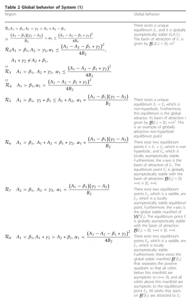
5 Global behavior
Theorem 18 Table 2describes the global behavior of System(1).
Proof. Throughout the proof of theorem≼will denote≼se.
(Ri,i= 1, 4)By Theorem 9,E1is locally asymptotically stable. ConsiderM(t) = (0,t)
fort≥ g2- A2. Since M(t)−T(M(t)) = −t+αA11,t(t+tA+2A−2γ2)
, we haveM(t)≼T(M(t)) for
t≥g2 -A2. By induction,TnM(t)≼Tn+1(M(t)))≼E1 for alln= 0,1,2,... becauseM(t)≼ E1for allt≥0. By monotonicity and boundedness, the sequence {Tn(M(t))} has to con-verge to the unique equilibrium E1. Consider N(u) = (u, 0) foru≥0. Lemma 3 implies
Tn(N(u))® E1 asn® ∞. Take any point (x,y)Î[0, +∞)×[0, +∞). Then there exists
t*, u* ≥ 0, such thatM(t*) ≼(x,y)≼(x,y)≼N(u*). The monotonicity of the mapT
impliesTn M(t*))≼Tn ((x, y))≼Tn(N(u*)). SinceTnM(t*)),Tn(N(u*))®E1as n® ∞, then Tn((x,y))®E1. This completes the proof.
(ℛ5) The first part of this theorem is proven in Theorem 9. The rest of the proof is
similar to the proof of part ((Ri,i= 1, 4)).
(ℛ6) By Lemma 3 y0 = 0 implies yn = 0, ∀nÎ N, and xn→ A1α−1β1, n® ∞, which shows thatx-axis is a subset of the basin of attraction ofE1.
Furthermore, every solution of (1) enters and stays in the box B(E2) and so we can restrict our attention to solutions that starts inB(E2). Clearly, the setQ2(E2)∩B(E2) is an invariant set with a single equilibrium point E2 and by Theorem 3, every solution that starts there is attracted to E2. In view of Corollary 1, the interior of rectangle
〚E2, E1〛is attracted to either E1 or E2, and becauseE2 is the local attractor, it is attracted to E2. If (x,y)∈A=B\([[E2,E1]]∪(Q2(E2)∩B)∪ {(x, 0) :x≥0}), then there exist the points (xu,yu)Î A∩Q4(E2) and (xl,yl)ÎQ2(E2)∩Bsuch that (xl, yl)
≼se(x,y)≼se(xu,yu). Consequently,Tn((xl,yl))≼seTn((x, y))≼seTn((xu,yu)) for alln = 1,2,... and soTn((x,y))® E2asn®∞, which completes the proof.
(ℛ7) The first part of this Theorem is proven in Theorem 13.
Now, we prove a global result.
JT(E1) =
β
1
A1 −
α1
A1(A1−β1) 0 (A1−β1)γ2
A1A2−β1A2+B2α1
(42)
The eigenvalues ofJT(E1) are given byλ1= βA11andλ2= A1A(2A−1β−1βA12+)γB22α1 and so
A2< γ2, α1< (
A1−β1) (γ2−A2)
B2 ⇒λ2>
1, A1> β1⇒λ1<1.
The eigenvector ofTatE1 that corresponds to the eigenvaluel1< 1 is (1, 0).
The rest of the proof is similar to the proof of part (ℛ6).
(ℛ8, ℛ9) The first part of theorem follows from Theorems 15 and 16. If parameters a1b1, A1, g2, A2andB2 do not satisfy the condition (8) of Lemma 1, then the mapT
defined on the set R=R2
Table 2 Global behavior of System (1)
Region Global behavior
R1A1> β1,A2< γ2<A1+A2−β1,
(A1−β1)(γ2−A2) B2 < α1≤
(A1−A2−β1+γ2)2
4B2
or
R2A1> β1,A2> γ2,α1≤
(A1−A2−β1+γ2)2 4B2
,
A1+γ2=A2+β1,
or
R3 A1> β1, A2=γ2, α1≤
(A1−A2−β1+γ2)2 4B2
or
R4 A1> β1,α1>
(A1−A2−β1+γ2)2 4B2
There exists a unique
equilibriumE1, and it is globally asymptotically stable (G.A.S.). The basin of attraction ofE1is given byB1(E1) = [0,∞)2
R5 A1> β1, γ2+β1≤A1+A2, α1=
(A1−β1)(γ2−A2) B2
There exists a unique equilibriumE1=E2which is non-hyperbolic. Furthermore, this equilibrium is the global attractor. Its basin of attraction is given byB(E1) = [0, +∞)2. This is an example of globally attractive non-hyperbolic equilibrium point
R6 A1> β1, A1+A2< β1+γ2, α1=
(A1−β1)(γ2−A2) B2
There exist two equilibrium pointsE=E1=E3which is non-hyperbolic, andE2, which is locally asymptotically stable. Furthermore, thex-axis is the basin of attraction ofE1. The equilibrium pointE2is globally asymptotically stable with the basin of attractionB(E2) = [0, +∞) × [0, +∞)
R7 A2> β1, A2< γ2, α1<
(A1−β1)(γ2−A2) B2
There exist two equilibrium pointsE1, which is a saddle, and
E2, which is a locally
asymptotically stable equilibrium point. Furthermore, thex-axis is the global stable manifold of
Ws(
E1). The equilibrium pointE2 is globally asymptotically stable with the basin of attraction
B(E2) = [0, +∞) × [0, +∞)
R8 A1< β1,A1+γ2>A2+β1,α1<
(A1−A2−β1+γ2)2 4B2
There exist two equilibrium pointsE3, which is a saddle, and
E2, which is locally asymptotically stable. Furthermore, there exists the global stable manifoldBs(E3)
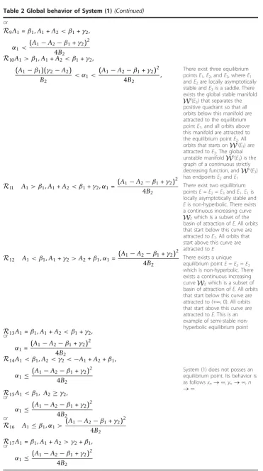
Table 2 Global behavior of System (1)(Continued)
or
R9A1=β1,A1+A2< β1+γ2,
α1< (A1−A2−β1+γ2)2 4B2
R10A1> β1,A1+A2< β1+γ2, (A1−β1)(γ2−A2)
B2 < α1<
(A1−A2−β1+γ2)2 4B2
,
There exist three equilibrium pointsE1,E2, andE3, whereE1 andE2are locally asymptotically stable andE3is a saddle. There exists the global stable manifold
Ws(
E3) that separates the positive quadrant so that all orbits below this manifold are attracted to the equilibrium pointE1, and all orbits above this manifold are attracted to the equilibrium pointE2. All orbits that starts onWs(E3) are attracted toE3. The global unstable manifoldWs(E3) is the graph of a continuous strictly decreasing function, andWu(E3)
has endpointsE2andE1
R11 A1> β1,A1+A2< β1+γ2,α1=
(A1−A2−β1+γ2)2 4B2
There exist two equilibrium pointsE=E2=E3andE1.E1is locally asymptotically stable and
Eis non-hyperbolic. There exists a continuous increasing curve
WEwhich is a subset of the
basin of attraction ofE. All orbits that start below this curve are attracted toE1. All orbits that start above this curve are attracted toE
R12 A1< β1,A1+γ2>A2+β1,α1=
(A1−A2−β1+γ2)2 4B2
There exists a unique equilibrium pointE=E2=E3 which is non-hyperbolic. There exists a continuous increasing curveWEwhich is a subset of
basin of attraction ofE. All orbits that start below this curve are attracted to (+∞, 0). All orbits that start above this curve are attracted toE. This is an example of semi-stable non-hyperbolic equilibrium point or
R13A1=β1,A1+A2< β1+γ2,
α1= (A1−A2−β1+γ2) 2
4B2
R14A1< β1,A2< γ2<−A1+A2+β1,
α1≤ (A1−A2−β1+γ2)2 4B2
System (1) does not posses an equilibrium point. Its behavior is as followsxn®∞,yn®∞,n
®∞ or
R15A1< β1, A2≥γ2,
α1≤ (A1−A2−β1+γ2)2 4B2
or
R16 A1≤β1,α1>
(A1−A2−β1+γ2)2 4B2
or
R17A1=β1,A1+A2> γ2+β1,
there exists the global stable manifoldWs(E3) that separates the first quadrant into two invariant regions W-(E3) (above the stable manifold) andW+(E3) (below the stable manifold) which are connected. Now, we show that each orbit starting in the region W+
(E3) is asymptotic to (∞,0). Indeed, setT1(x,y) = α1+β1x
A1+y ,T2(x,y) =
γ2y
A2+B2x+y. Takex=
(x0,y0)ÎW+(E3)∩ℛ(+, -), where ℛ(+, -) = {(x,y)Î ℛ:T1(x, y) >x,T2(x,y) <y}. As is known, see [12], the setℛ(+, -) is invariant. We have
T1(x0,y0) = α1+β1x0 A1+y0 >
x0, T2(x0,y0) = γ2y0 A2+B2x0+y0 <
y0,
which implies the following
(x0,y0)se(T1(x0,y0),T2(x0,y0))⇔(x0,y0)seT(x0,y0).
By monotonicity, T(x0, y0)≼seT2 (x0, y0) and by induction,Tn(x0, y0)≼seTn+1 (x0,
y0). This implies that sequence {xn} is non-decreasing and {yn} is non-increasing. Since, {yn} is bounded from above, hence it must converges. Now limn®∞yn= 0 since other-wise (xn,yn) will converge to another limit which is strictly south-east ofE3, which is impossible. By Lemma 3,xn®∞. By Theorems 6-8 for all (x,y)ÎW+(E3), there exists
n0 > 0 such thatTn((x,y))Î int(Q4(E3)∩ℛ),n>n0. We see that for all (x,y)Î int(Q4
(E3))∩ℛ), there exists (xl,yl)ÎW+(E3)∩ℛ(+, -) such that (xl,yl)≼(x,y). By mono-tonicityTn((xl,yl))≼Tn((x,y)) ≼(∞, 0). This impliesTn((x,y))®(∞, 0) asn®∞.
Now, we show that each orbit starting in the region W-(E3) converges toE2. By The-orem 6, for all (x, y)ÎW-(E3), there existsn0 > 0 such that,Tn((x,y))Î int(Q2(E3)∩ ℛ), n >n0. Set M(t) = (0, t) By part ((Ri,i= 1, 4)), for t ≥ g2 - A2, we have
M(t)T(M(t))E2.. By using monotonicity,Tn(M(t))®E2as n® ∞. By Corollary 1, the interior of rectangle 〚E2, E3〛is attracted to eitherE2 orE3, and becauseE2 is local attractor, it is attracted to E2. If (x, y) Î int(Q2(E3)∩ ℛ), then there exist the points (xr, yr)Î 〚E2,E3〛andt* ≥g2- A2, such thatM(t*)≼se (x,y)≼se(xr, yr). Con-sequently,Tn(M(t*))≼seTn((x,y))≼seTn((xr,yr)) for alln= 1, 2,... and soTn((x,y))®
E2asn®∞.
Now, assume that parametersa1, b1, A1, g2, A2, andB2 satisfy the condition (8) and
inequality 1.i) of Lemma 1. Then the set
I=
x,A1A2β1+xA1B2β1 B2α1−A2β1
:x≥0
is invariant and contains the equilibrium point E3, andT(x, y) =E3for (x, y)Îℐ. In view of the uniqueness of global stable manifold, we conclude that Ws(E3) =ℐ. Take any point (x, y)Î W+(E3). Then there exists the point (xl,yl)Î ℐ such that (xl, yl) <<se(x, y). Since, the mapT is strongly competitive, thenE3 =T(xl, yl) <<seT(x,y). This impliesT(x,y)Î int(Q4(E3)∩ℛ). Similarly, if (x,y)ÎW-(E3), thenT(x, y)Îint
(Q2(E3)∩ ℛ). The rest of the proof is similar to the proof of the first case. This com-pletes the proof.
(ℛ10) The first part of the theorem follows from Theorem 10. If parametersa1,b1, A1,g2,A2, and B2 do not satisfy the condition (8) of Lemma 1, then the mapT, defined
on the setR=R2
+,, satisfies all conditions of Theorems 4, 6-8. This implies that there exists the global stable manifold Ws(
invariant regions W+(E3) (below the stable manifold) andW-(E3) (above the stable manifold) which are connected.
Using Theorems 6, 7, and 8, we have that for all (x, y)ÎW+(E3), there exists n0>0 such that for n > n0, Tn((x, y))Î int(Q4(E3)∩ ℛ), and for all (x, y) ÎW-(E3), there exists n1 >0 such that for alln > n1,Tn((x,y))Î int(Q2(E3)∩ℛ). Now, we show that each orbit starting in the region int(Q4(E3)) converges toE1, and each orbit starting in the regionint(Q2(E3)) converges toE2.
Take 0≤t≤(g2-A2)/B2, U(t) = (t,-A2 -tB2+g2). It is easy to see that the following holds
U(x¯) =E=E2=E3E1 wherex¯=x2=x3 and
U(t)−T(U(t)) =
−(−A1+A2+ 2tB2+β1−γ2)2 4B2(A1−A2−tB2+γ2)
, 0
.
Since x2 andx3are solutions of the equationB2t2 + (-A1+A2 +b1- g2)t+a1= 0
and the following inequality holds A2 +tB2 -g2<0, we have thatU(t)≼se T(U(t)) for 0
≤t≤x2and x3≤t≤(g2 -A2)/B2 andT(U(t)))≼seU(t) forx2 ≤t≤x3.
By using monotonicity ofT, we have that for 0≤t < x2,Tn(U(t))≼Tn+1(U(t))≼E2, and for x2 ≤t < x3,E2 ≼Tn+1(U(t))≼Tn(U(t))≼E3. This implies Tn(U(t))® E2 as n ® ∞. Similarly, forx3 ≤t≤(g2- A2)/B2, we haveE3≼Tn(U(t))≼Tn+1(U(t)) ≼E1. This
implies Tn(U(t))® E1 asn® ∞. By using the property of points U(t) andN(u), we have that for each point (x, y)Îint(Q4(E3)∩ ℛ), there exitsx3 < t* <(g2 -A2)/B2 and u*>0 such thatU(t*) ≼(x,y)≼N(u*). By using monotonicity ofT, we haveTn(U(t*))
≼ Tn((x, y)) ≼Tn(N(u*))). This implies Tn((x, y)) ® E1 asn® ∞. Furthermore, for each point (x, y)Î int(Q2(E3)∩ℛ), there existt1 >0 andt2,x2 < t2< x3 such thatM
(t1)≼(x, y)≼U(t2). By using monotonicity ofT, we haveTn(M(t1))≼Tn((x,y))≼Tn
(U(t2)). This impliesTn((x,y)) ®E2 asn® ∞.
Now, assume that parameters a1, A1, g2, A2, and B2 satisfy the condition (8) and
inequality 1.i) of Lemma 1. Then the set
I=
x,A1A2β1+xA1B2β1 B2α1−A2β1
:x≥0
is invariant and contains the equilibrium pointE3 andT(x,y) = E3 for (x,y)Î I. In view of the uniqueness of global stable manifold, we conclude that Ws(E3) =ℐ. Take any point (x,y)ÎW+(E3), then there exists the point (xl,yl)Îℐsuch that (xl, yl) <<se (x,y). Since, the map Tis strongly competitive, then E3 =T(xl, yl) <<seT(x,y). This implies T(x, y)Î int(Q4(E3)∩ℛ). Similarly, if (x, y)ÎW-(E3), thenT(x,y)Î int(Q2
(E3)∩ℛ). The rest of the proof is similar to the proof of the first case. This completes the proof.
(ℛ11) The first part of theorem follows from Theorems 15 and 16. If parametersa1, b1, A1,g2, A2, and B2 do not satisfy the condition (8) of Lemma 1, then the map T,
defined on the set R=R2
By Theorems 6 and 7 and 8 for all (x, y)Î W+(E), there exists n0 > 0 such thatTn
((x,y))Îint(Q4(E)∩ℛ) for n>n0. For all (x,y)ÎW-(E), there existsn1> 0 such that for alln>n1,Tn((x,y)) Îint(Q2(E)∩ℛ). Now, we show that each orbit starting in the regionint(Q4 (E)) converges toE1, and each orbit starting in the regionint(Q2(E)) con-vergesE.
Now, for 0≤t≤(g2-A2)/B2, takeU(t) = (t,-A2 -tB2 +g2) Sincea1= (A1-A2- b1+ g2
)2/(4B2), it is easy to see that the following holds
U(x¯) =E=E2=E3E1 wherex¯=x2=x3 and
U(t)−T(U(t)) =
−(−A1+A2+ 2tB2+β1−γ2)2 4B2(A1−A2−tB2+γ2)
, 0
.
Since A2+tB2- g2< 0, we haveU(t)seT(U(t))for 0≤t≤(g2- A2)/B2.
By using monotonicity of T, we have thatTn(U(t))Tn+1(U(t))Efor0≤t<¯x. This implies Tn(U(t)) ® E as n ® ∞. Similarly, for x¯≤t<(γ2−A2)/B2, ETn(U(t))Tn+1(U(t))E
1. This implies Tn(U(t))®E1 asn® ∞. By using the property of the points U(t) andN(u), we have that for each point (x, y)Î int(Q4(E)∩ ℛ), there exist x¯<t∗<(γ2−A2)/B2and u* > 0 such thatU(t∗)(x,y)N(u∗). By using monotonicity of T, we have that Tn(U(t∗))Tn((x,y))Tn(N(u∗))).This impliesTn((x,y))® E1asn®∞. Furthermore, for each point (x,y)Îint(Q2(E)∩ℛ) there exists t1 > 0 such thatM(t1)(x,y)E. By using monotonicity of T, we have Tn(M(t1))Tn((x,y))E. This impliesTn((x,y))® Easn®∞.
Now, assume that parametersa1, b1, A1, g2, A2, andB2 satisfy the condition (8) and
inequality 1.i) of Lemma 1. The proof of Theorem is similar to the proof of Theorem in the regions (ℛ9) and (ℛ10).
(ℛ12, ℛ13) The first part of theorem follows from Theorems 15 and 17. If
para-metersa1,b1,A1g2,A2, andB2 do not satisfy (8) of Lemma 1, then the mapT, defined
on the setR=R2
+,satisfies all conditions of Theorems 4,6, and 8. This implies that there exists an invariant curve C, which is a subset of the basin of attraction of the equilibrium pointE, and which separates the first quadrant into two invariant regions, W+
(E) (below the stable manifold) andW-(E) (above the stable manifold) which are connected.
By Theorems 6 and 8 for all (x,y)ÎW+(E), there exists n0> 0 such thatTn((x,y))Î
int(Q4(E)∩ℛ) for n>n0, and for all (x,y)Î C-(E), there existsn1> 0 such thatTn((x,
y))Î int(Q2(E)∩ℛ) for alln>n1. Now, we show that each orbit starting in the region
int(Q4(E)) is asymptotic to (∞, 0) and each orbit starting in the regionint(Q2(E)) con-verges to E.
Sincea1= (A1- A2b1 +g2)2/(4B2), for 0≤t≤(g2 -A2)/B2, we haveU(t) = (t, -A2 -tB2+g2). It is easy to see
U(x¯) =E=E2=E3 wherex¯=x2=x3 and
U(t)−T(U(t)) =
−(−A1+A2+ 2tB2+β1−γ2)2 4B2(A1−A2−tB2+γ2)
, 0
.
Since A2+tB2- g2< 0, for 0≤t≤(g2-A2)/B2, we haveU(t)seT(U(t)). By using monotonicity of T, we haveETn(U(t))Tn+1(U(t))E
10≤t<x. This¯ implies Tn(U(t)) ® E asn ® ∞. Similarly, ETn(U(t))Tn+1(U(t))(∞, 0)for
¯
Î int(Q4(E3) ∩ ℛ), there exists x¯<t∗ <(γ2−A2)/B2 such that 0≤t<x.¯ 0≤t<x. By monotonicity of¯ T, we have Tn(U(t∗))Tn((x,y))(∞, 0). This implies Tn((x,y)) ®(∞, 0) asn® ∞. Furthermore, for each point (x,y)Î int(Q2
(E3)∩ℛ), there existst1 > 0 such thatU(t∗)(x,y)N(u∗). By monotonicity ofT, we haveTn(M(t1))Tn((x,y))E. This impliesTn((x,y)) ®Easn®∞.
If parameters a1,b1, A1,g2,A2, andB2 satisfy the condition (8) and inequality 1.i) of
Lemma 1, then the proof of Theorem is similar to the proof of parts (ℛ9) and (ℛ10).
This completes the proof of Theorem in the regions ℛ12,ℛ13. This is an example of
semistable non-hyperbolic equilibrium point.
Ri,i= 14, 17
Assumptions of this theorem imply that equilibrium does not exist.
Set M (t) = (0, t) for t≥ g2 - A2. Since M(t)−T(M(t)) =
− α1
t+A1
,t(t+A2−γ2) t+A2
,
we haveM(t)≼T(M(t)) for t≥ g2- A2. By using monotonicityTn(M(t))≼Tn+1(M(t))),
for alln= 0, 1, 2,... Set(x∗n,yn∗) =Tn(M(t)). This implies that{y∗
n}is non-increasing and bounded, hence it has to converge. Setlimn→∞y∗n=y∗. Since{x∗n}is unbounded and non-decreasing, we have thatx∗n→ ∞. By using the second equation of the System (1), we see thaty∗= 0. Take any point (x,y)Î [0,∞)2. Then there exists t*, such thatM
(t*) ≼(x,y)≼(∞, 0). By using monotonicity,Tn(M(t*))≼(Tn((x,y))≼(∞, 0) as Since
Tn(M(t*))®(∞, 0) asn® ∞, we obtainTn((x,y))® (∞, 0) asn®∞, as which com-pletes the proof of theorem.
Author details
1
Department of Mathematics, University of Sarajevo, Sarajevo, Bosnia and Herzegovina2Department of Mathematics, University of Rhode Island, Kingston, RI 02881-0816, USA
Authors’contributions
All authors contributed equally to the manuscript and read and approved the final draft.
Competing interests
The authors declare that they have no competing interests.
Received: 26 January 2011 Accepted: 23 August 2011 Published: 23 August 2011
References
1. Camouzis, E, Kulenović, MRS, Ladas, G, Merino, O: Rational systems in the plane. J Differ Equ Appl.15, 303–323 (2009). doi:10.1080/10236190802125264
2. Kulenović, MRS, Merino, O: Invariant manifolds for competitive discrete systems in the plane. Int J Bifurcat Chaos.20, 2471–2486 (2010). doi:10.1142/S0218127410027118
3. Kulenović, MRS, Merino, O: Global bifurcation for competitive systems in the plane. Discret Cont Dyn Syst B.12, 133–149 (2009)
4. AlSharawi, Z, Rhouma, M: Coexistence and extinction in a competitive exclusion Leslie/Gower model with harvesting and stocking. J Differ Equ Appl.15, 1031–1053 (2009). doi:10.1080/10236190802459861
5. Cushing, JM, Levarge, S, Chitnis, N, Henson, SM: Some discrete competition models and the competitive exclusion principle. J Differ Equ Appl.10, 1139–1152 (2004). doi:10.1080/10236190410001652739
6. Kulenović, MRS, Nurkanović, M: Asymptotic behavior of a linear fractional system of difference equations. J Inequal Appl. 127–143 (2005)
7. Clark, D, Kulenović, MRS, Selgrade, JF: Global asymptotic behavior of a two dimensional difference equation modelling competition. Nonlinear Anal TMA.52, 1765–1776 (2003). doi:10.1016/S0362-546X(02)00294-8
8. Hirsch, MW: Systems of differential equations which are competitive or cooperative. I Limits Sets SIAM J Math Anal.
13(2):167–179 (1982)
9. Hirsch, M, Smith, H: Monotone dynamical systems. In: Canada A, Drabek P, Fonda A (eds.) Handbook of Differential Equations: Ordinary Differential Equations, vol. II, pp. 239–357. Elsevier, Amsterdam (2005)
10. Kalabušić, S, Kulenović, MRS, Pilav, E: Global dynamics of a competitive system of rational difference equations in the plane. Adv Differ Equ 30 (2009). Article ID 132802
11. Kulenović, MRS, Merino, O: Discrete Dynamical Systems and Difference Equations with Mathematica. Chapman & Hall/ CRC Press, Boca Raton (2002)
13. Leonard, WJ, May, R: Nonlinear aspects of competition between species. SIAM J Appl Math.29, 243–275 (1975). doi:10.1137/0129022
14. Smith, HL: Invariant curves for mappings. SIAM J Math Anal.17, 1053–1067 (1986). doi:10.1137/0517075
15. Smith, HL: Periodic competitive differential equations and the discrete dynamics of competitive maps. J Differ Equ.64, 165–194 (1986). doi:10.1016/0022-0396(86)90086-0
16. Smith, HL: Periodic solutions of periodic competitive and cooperative systems. SIAM J Math Anal.17, 1289–1318 (1986). doi:10.1137/0517091
17. Smith, HL: Planar competitive and cooperative difference equations. J Differ Equ Appl.3, 335–357 (1998). doi:10.1080/ 10236199708808108
18. Smith, HL: Non-monotone systems decomposable into monotone systems with negative feedback. J Math Biol.53, 747–758 (2006). doi:10.1007/s00285-006-0004-3
19. Takáč, P: Domains of attraction of genericω-limit sets for strongly monotone discrete-time semigroups. J Reine Angew Math.423, 101–173 (1992)
20. de Mottoni, P, Schiaffino, A: Competition systems with periodic coefficients: a geometric approach. J Math Biol.11, 319–335 (1981). doi:10.1007/BF00276900
21. Hess, P: Periodic-Parabolic Boundary Value Problems and Positivity. In Pitman Research Notes in Mathematics Series, vol. 247,Longman Scientific & Technical, Harlow (1991)
22. Kocic, V, Ladas, G: Global Behavior of Nonlinear Difference Equations of Higher Order with Applications. Kluwer, Dordreht (1993)
doi:10.1186/1687-1847-2011-29
Cite this article as:Kalabušićet al.:Dynamics of a two-dimensional system of rational difference equations of Leslie–Gower type.Advances in Difference Equations20112011:29.
Submit your manuscript to a
journal and benefi t from:
7 Convenient online submission 7 Rigorous peer review
7 Immediate publication on acceptance 7 Open access: articles freely available online 7 High visibility within the fi eld
7 Retaining the copyright to your article