ORDERING ON TIME SCALES
PETR STEHL´IKReceived 31 January 2006; Revised 16 May 2006; Accepted 16 May 2006
In order to enlarge the set of boundary value problems on time scales, for which we can use the lower and upper solutions technique to get existence of solutions, we extend this method to the case when the pair lacks ordering. We use the degree theory and a priori estimates to obtain the existence of solutions for the second-order Dirichlet boundary value problems. To illustrate a wider application of this result, we conclude with an ex-ample which shows that a combination of well- and nonwell- ordered pairs can yield the existence of multiple solutions.
Copyright © 2006 Petr Stehl´ık. This is an open access article distributed under the Cre-ative Commons Attribution License, which permits unrestricted use, distribution, and reproduction in any medium, provided the original work is properly cited.
1. Introduction
The method of lower and upper solutions is a widely used concept in the study of nonlin-ear boundary value problems (further abbreviated by BVP). Three quarters of the century after the pioneering work of Dragoni [8] this method still belongs among the basic tools and is frequently employed in applied analysis or mechanics. Dragoni’s basic idea was to transform the BVP with an unbounded right-hand side into a problem with a bounded right-hand side (this transformation is possible thanks to the existence of lower and upper solutions) and, in the second step, to show that a solution of the modified problem is also a solution of the original problem. Together with the later introduced Nagumo conditions for the derivative dependent right-hand sides this basic scheme forms the foundations of this method.
On the other hand, the time scales calculus, with its concept to unify and extend dis-crete and continuous worlds, is a recent idea (the seminal work is due to Hilger, see, e.g., [9]). In spite of this, this calculus is already broadly used. It is not surprising that, af-ter the Schauder fixed point theorem for bounded right-hand sides, the lower and upper solutions technique was used to investigate the problems with unbounded right-hand sides. The first results for Dirichlet boundary conditions are due to Akin [2], or Bohner
Hindawi Publishing Corporation Advances in Difference Equations Volume 2006, Article ID 73860, Pages1–12
and Peterson [3, Section 6.6]. Later, similar statements were obtained also for periodic conditions, see, for example, Cabada [5], Stehl´ık [12], or Topal [13].
The main drawback of the concept of lower and upper solutions, which often hinders its practical application, is the assumption on their existence. Logical reaction to this objection was a successful attempt to include also the case when the lower and upper solutions do not satisfy the common ordering, that is, the lower solution is above the upper solution in some points of the considered interval. The so-called nonwell-ordered case for differential equations was first studied in 1970s, see, for example, Sattinger [11].
The traditional ways to deal with the nonwell-ordered pairs rely on the periodicity and boundedness of trigonometric functions, properties of Fuˇc´ık spectrum and the existence of intersections of lower and upper solutions (for the survey on lower and upper solu-tions, see, e.g., De Coster and Habets [6]). Unfortunately, one cannot straightforwardly extend these concepts to the discrete or time scales context. Therefore, we avoid these approaches by relying on the degree theory.
We recall the basic definitions and notations concerning time scales calculus, the reader acquainted with the basic concepts (within the scope of the first chapters of Bohner and Peterson [3,4]) can jump over to (1.6).
Time scaleTis an arbitrary nonempty closed subset of the real numbersR. The natural numbersN, the integersZ, or the union of intervals [0, 1]∪[2, 3] are the most natural examples.
Fort∈Twe define theforward jump operatorσ:T→Tand thebackward jump oper-atorρ:T→Tby
ρ(t) :=inf{s∈T:s > t}, ρ(t) :=sup{s∈T:s < t}, (1.1)
where we put inf∅ =supTand sup∅ =infT. We say that a pointt∈Tisright-scattered, left-scattered,right-dense, left-denseifσ(t)> t,ρ(t)< t, σ(t)=t,ρ(t)=t, respectively. Moreover, we define theforward graininessfunctionμ:T→[0,∞) by
μ(t) :=σ(t)−t. (1.2)
In the above references one can find the definition of the so-calleddelta-derivativexΔ, which is equivalent tox ifT=R, or toΔx ifT=Z. Similarly, several concepts of in-tegration have been extended as well, ranging from Cauchy-Newton [3, Section 1.4] to Henstock-Kurzweil [10] integration.
For the sake of clarity we introduce the closed time scale interval by
[a,b]T=[a,b]∩T, (1.3)
with the note that other types of intervals are defined in the analogous way. To simplify complicated formulae, we use the abridged notations
We define an rd-continuousfunction as a function that is continuous in all right-dense points and left-sided limits exist in left-dense points. The set of all rd-continuous func-tions will be denoted byCrd. The set of twice differentiable functions whose second de-rivative is rd-continuous will be denoted byC2
rd. Finally, we define the following function space:
Crd,02
0,σ2(1)T:=x∈Crd2 :x(0)=x
σ2(1)=0. (1.5)
For the sake of brevity, we often useC2
rd,0instead.
In this paper we consider a nonwell-ordered couple of lower and upper solutions for the following Dirichlet BVP:
−xΔΔ(t)= ft,xσ(t) on [0, 1]T
x(0)=xσ2(1)=0. (1.6)
The solution of (1.6) is a functionx∈C2rd,0which satisfies the equation for allt∈[0, 1]T. We base our work on the existence theorems for the well-ordered case which are pre-sented in Akin [2]. Therefore, we start, inSection 2, with a slight modification of one of these results. Namely, we provide further information about the degree of the corre-sponding operator.
Next, inSection 3, we use this extension to prove the existence in nonwell-ordered set-ting. Aside from the degree theory, a priori estimate and the properties of first eigenvalue and eigenfunction are our main tools. If f satisfies certain growth and limit conditions, we obtain the existence of a solution. The similar approach for thep-Laplacian can be found in Dr´abek et al. [7].
Finally, by combining these results we suggest how to acquire the existence of multiple solutions. This idea is illustrated, inSection 4, on the existence of three solutions.
2. Well-ordered case
In this section we present the basic definitions and notations for lower and upper solu-tions and we amend the existing results for well-ordered pairs. Let us first define lower and upper solutions for BVP (1.6).
Definition 2.1. A functionα∈Crd2([0,σ2(1)]T) is called alower solutionof (1.6) if
α(0)≤0, ασ2(1)≤0,
−αΔΔ(t)≤ft,ασ ∀t∈0,σ2(1)T. (2.1)
Similarly, a functionβ∈C2
rd([0,σ2(1)]T) is called anupper solutionof (1.6) if
β(0)≥0, βσ2(1)≥0, −βΔΔ(t)≥ft,βσ ∀t∈0,σ2(1)
T.
(2.2)
Definition 2.2. A functionxis strictly smaller thany(denoted byxy) if
x(t)< y(t) fort∈0,σ2(1)T, (2.3)
and the following conditions hold on the boundary: (i) eitherx(0)< y(0), orxΔ(0)< yΔ(0), and
(ii) eitherx(σ2(1))< y(σ2(1)), orxΔ(σ(1))< yΔ(σ(1)).
Using this ordering we can define an important subclass of lower and upper solutions. Definition 2.3. A functionαis astrictlower solution of (1.6) if
(i)αis a lower solution of (1.6),
(ii) every possible solutionxof (1.6) satisfyingα≤xsatisfiesαx.
Reversing the above inequality we can get the corresponding definition of astrictupper solution.
As usual, we introduce the solution operatorT:C2
rd,0→C2rd,0defined by At this stage, we are ready to state an expanded existence theorem.
Theorem2.4. Let f be a continuous function. Letα,βbe lower and upper solutions, respec-tively, for whichα≤βholds. Then the problem (1.6) has at least one solutionxsatisfying
α≤x≤β in0,σ2(1)
Proof. With the purpose of applying the Schauder fixed point theorem, Bohner and Pe-terson, in [3, Theorem 6.54], define a modified right-hand side function by
f(t,x)=
Using the continuity and boundedness of this function, it obtains the compactness ofT
operator. Finally, one can show thatα(t)≤x(t)≤β(t) which implies thatxis also the fixed point ofTdefined by (2.4) and thus a solution of (1.6).
We define the constantR0>0 as a bound of operatorT(the existence of this bound is ensured by the definition of f), that is, for eachy∈C2rd,0we have
T(y)C2
rd,0< R0. (2.9) This guarantees the existence of an admissible homotopy:
H(τ,x)=I(x)−τT(x) τ∈[0, 1], (2.10)
which implies the following equality of degrees:
degI−T;Bo,R0
,o=degI;Bo,R0
,o=1. (2.11)
Moreover, sinceαandβare strict, there is no solution ofx=T(x) withx(t)≤α(t) or
x(t)≥β(t) for anyt∈(0,σ2(1))
Tand we can deduce that
degI−T;Ω1,o
=degI−T;Bo,R0
,o=1. (2.12)
To conclude, the definition ofΩ1yields that
degI−T;Ω1,o
=degI−T;Ω1,o
=1. (2.13)
3. Nonwell-ordered case
First of all, we recall the basic results concerning the eigenvalue problem:
−xΔΔ(t)=λx(t) on0,σ2(1) T,
x(0)=xσ2(1)=0. (3.1)
Using the existing oscillation theorem we can prove this simple statement.
Lemma3.1. The first eigenvalueλ1of (3.1) is positive and the corresponding eigenfunction
ϕ1(t)>0for allt∈(0,σ2(1))T.
Proof. Obviously, (3.1) has only a trivial solution ifλ=0. Now, let us suppose thatλ <0 is an eigenvalue. The corresponding eigenfunctionϕ(t) (or−ϕ(t)) must attain a maximum in (0,σ2(1))
T. Let us suppose thatm∈(0,σ2(1))Tis the first point where the maximum is attained. Let us distinguish between two cases.
(i)mis left-dense. In that caseϕΔΔ(m)≤0 andϕΔ(m)=0, which leads to the fol-lowing contradiction:
(ii)m is left-scattered. This implies thatxΔ(m)≤0 andxΔ(ρ(m))>0 and we can
The positivity of first eigenfunctions is the immediate consequence of oscillation theo-rem, which is due to Agarwal et al. [1, Theorem 1] or Bohner and Peterson [3, Theorem
4.106].
At this stage, we are ready to prove the existence result also in the case when lower and upper solutions are without ordering.
Theorem3.2. Let f be a continuous function satisfying that (i)there arec,d >0such that
Proof. We assume that there is no solution on∂S(otherwise there is no reason to proceed with the proof). For the sake of lucidity, we divide our proof into three parts.
then there existsK >0 such that for anyr >0 and any solutionx∈Sof
−xΔΔ(t)= fr
t,xσ(t) on [0, 1]T,
x(0)=xσ2(1)=0, (3.10)
the following a priori estimate holds:
xC2
rd,0≤K. (3.11)
As usual, we suppose that this assumption is not satisfied, that is, there exists a sequence {rk}∞k=1 with rk >0 and a corresponding sequence of solutions {xk}∞k=1 satisfying
The boundedness of the sequence (clearlyykC2
rd,0 =1) and the compactness ofT pro-vide convergence (at least for a subsequence) to somey∈C2
rd,0
yk−→y inCrd,02 . (3.14)
The condition (3.4) implies that for some sufficiently largeε≥0 the right-hand sides of (3.13) are bounded by a constant (and thus integrable) functionh(s)=d+εand, more-over, using the limit assumption (3.5) we can get
frk
Thus the dominated convergence theorem (see Peterson, Thompson [10, Theorem 2.17] for its most general form on time scales) yields thatysolves the problem:
−yΔΔ(t)=λ1y(t) on [0, 1]T,
y(0)=yσ2(1)=0. (3.16)
Similarly, if yis negative, then there isk∈Nsuch that for allk > k0and for allη∈ (0,σ2(1))
Twe havex(η)< β(η), a contradiction.
(ii) Construction of strict well-ordered lower and upper solutions. Let us consider an arbitraryR >0 satisfying
R > R0:=max
K,αC,βC+ 1, (3.17)
and the BVP (3.10) withr=R, that is,
−xΔΔ(t)= fRt,xσ(t) on [0, 1]T,
x(0)=xσ2(1)=0. (3.18)
We show thatu:= −R−2 andv:=R+ 2 are lower and upper solutions of (3.18), respec-tively. Obviously,uis a lower solution since
u(0)= −R−2<0, uσ2(1)= −R−2<0,
uΔΔ(t)=0= fR(t,−R−2), ∀t∈[0, 1]T.
(3.19)
Now assume thatuis not strict, that is, there existsm∈(0,σ2(1))
Tdefined by
m:= min t∈(0,σ2(1))
T
t:x(t)= −R−2. (3.20)
Again, we divide our reasoning into two parts.
(a) Let us suppose thatmis left-dense. The minimality ofxatmimplies thatxΔ(m)= 0 and the left-density ofmprovides the existence ofε >0 such thatx(t)<−R−1 for allt∈(m−ε,m)T, that is, fR(t,xσ(t))=0 for theset. These two facts suggest thatxΔΔ(t)=0 for allt∈[m, 1]T. Thusx(σ2(1))= −R−2 andxis not a solution of (3.18), a contradiction.
(b) Now, we assume thatmis left-scattered. Sincexachieves its minimum first atm, we obtain the following two conditions:
xΔ(m)≥0, xΔρ(m)<0. (3.21)
But this leads to the following contradiction:
0=fR
ρ(m),x(m)=xΔΔρ(m)=xΔ(m)−xΔ
ρ(m)
μρ(m) >0. (3.22)
Similarly, one can derive thatv=R+ 2 is a strict supersolution of (3.18). (iii)Computation of the degree. We defineTR:C2rd,0→Crd,02 by
TR(x) := σ(1)
0 G(t,s)fR
s,xσ(s). (3.23)
Obviously, if we find a fixed pointx0ofTR, thenx0is a solution of (3.18). If, moreover,
β(t)
α(t)
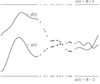
v(t)=R+ 2
u(t)=R2
Figure 3.1. Nonwell-ordered case.
operatorsTandTRcoincide on this ball. We define three sets by
Ωv u:=
x∈C2
rd,0:uxv
,
Ωv α:=
x∈Crd,02 :αxv
, Ωβu:=x∈Crd,02 :uxβ
. (3.24)
Clearly,Ωv
α,Ωβu, andΩ2are pairwise disjoint subsets. Thus the properties of the degree and the well-ordered result (Theorem 2.4) enable the following computation:
1=degI−TR;B(o,R)∩Ωvu,o
=degI−TR;B(o,R)∩Ωβu,o
+ degI−TR;B(o,R)∩Ωvα,o
+ degI−TR;Ω2,o =2 + degI−TR;Ω2,o
.
(3.25)
Therefore (TandTRcoincide onB(o,R)), we obtain the required result:
degI−T;Ω2,o
= −1. (3.26)
The statement ofTheorem 3.2and the strict pairuandvfrom its proof are illustrated inFigure 3.1.
Remark 3.3. In contrast toTheorem 2.4,Theorem 3.2gives less transparent information about the existing solution. This is mainly due to the opaque structure ofS(and conse-quently ofΩ2). In fact, we know only that there exists a boundRon the norm of this solution (Ris closer specified in the proof in (3.17)) and that there existξ,η∈(0,σ2(1))
T such thatx(ξ)< α(ξ) andx(η)> β(η), respectively.
Example 3.4. Let us deal withT=(1/5)Zand a continuous function
Clearly, f satisfies conditions (i) and (ii) ofTheorem 3.2. Let us consider the correspond-ing BVP:
β(t). Therefore, we can applyTheorem 3.2and claim that the problem (3.28) has a so-lutionx∈C2
rd,0. The only additional information about this solution is that there exist
ξ,η∈[1/5, 6/5]Tsuch thatx(ξ)≤α(ξ) andx(η)≥β(η).
4. Multiple solutions
The combination of the results for well-ordered case and nonwell-ordered counterpart opens the way for the existence of multiple solutions. As an example of such a process we state a simple result for the existence of three solutions, which can be generalized to other cases.
Theorem4.1. Let f satisfy the assumptions(i)and(ii)fromTheorem 3.2. Assume thatα1 andα2are lower solutions andβ1andβ2are upper solutions of (1.6) which satisfy
α1β1, α2β2, (4.1)
and assume that there existτ∈(0,σ2(1))
Tsuch that
α2(τ)> β1(τ). (4.2)
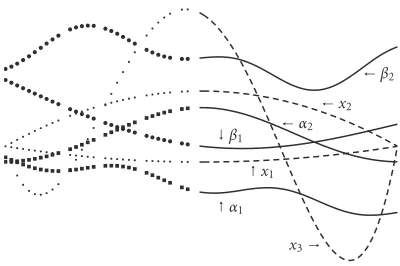
β1
α1 x1
α2
x3 x2
β2
Figure 4.1. Existence of three solutions.
Proof. First, we apply twiceTheorem 2.4to obtain the existence of solutionsx1 andx2 satisfying
α1x1β1, α2x2β2. (4.3)
Furthermore, (4.2) allows us to applyTheorem 3.2to obtain the existence of a solution
x3. Sincex3∈S, we know that there existsξ,η∈(0,σ2(1))Tsuch thatx3(ξ)≤α2(ξ) and
x3(η)≥β1(η) and this implies thatx3is different tox1,x2. The statement ofTheorem 4.1 and the solutionsxi,i= {1, 2, 3}, from its proof are illustrated inFigure 4.1.
Theorem 4.1basically claims that if you have a nonwell-ordered couple and for each function from this pair you are able to find a function with which it forms an ordered cou-ple, you have at least three solutions. We illustrate this idea on the extension ofExample 3.4.
Example 4.2. Let us assume that f,α, andβare defined as inExample 3.4. Obviously
α(t)≡ −5 and β(t)≡5 are another lower and upper solutions of (3.28) (note that
f(t,±5)=0). Thus we can claim that the problem (3.28) has at least three distinct so-lutions wherex3is described inExample 3.4,αx1βandαx2β.
Acknowledgments
The author gratefully acknowledges the support of the Ministry of Education, Youth and Sports of the Czech Republic, Research Plan no. MSM 4977751301. Moreover, he is also obliged to Pavel Dr´abek, Bevan Thompson, and Milan Tvrd´y for their valuable hints and suggestions.
References
[1] R. P. Agarwal, M. Bohner, and P. J. Y. Wong,Sturm-Liouville eigenvalue problems on time scales, Applied Mathematics and Computation99(1999), no. 2-3, 153–166.
[3] M. Bohner and A. Peterson,Dynamic Equations on Time Scales. An Introduction with Applica-tions, Birkh¨auser Boston, Massachusetts, 2001.
[4] M. Bohner and A. Peterson (eds.),Advances in Dynamic Equations on Time Scales, Birkh¨auser Boston, Massachusetts, 2003.
[5] A. Cabada,Extremal solutions and Green’s functions of higher order periodic boundary value prob-lems in time scales, Journal of Mathematical Analysis and Applications290(2004), no. 1, 35–54. [6] C. De Coster and P. Habets,The lower and upper solutions method for boundary value problems,
Handbook of Differential Equations (A. Ca˜nada, P. Dr´abek, and A. Fonda, eds.), Elsevier/North-Holland, Amsterdam, 2004, pp. 69–160.
[7] P. Dr´abek, P. Girg, and R. Man´asevich,Generic Fredholm alternative-type results for the one di-mensionalp-Laplacian, Nonlinear Differential Equations and Applications8(2001), no. 3, 285– 298.
[8] G. S. Dragoni,II problema dei valori ai limiti studiato in grande per le equazioni differenziali del secondo ordine, Mathematische Annalen105(1931), no. 1, 133–143.
[9] S. Hilger,Analysis on measure chains—a unified approach to continuous and discrete calculus, Results in Mathematics18(1990), no. 1-2, 18–56.
[10] A. Peterson and H. B. Thompson,The Henstock-Kurzweil delta and nabla integrals, to appear in Journal of Mathematical Analysis and Applications.
[11] D. H. Sattinger,Monotone methods in nonlinear elliptic and parabolic boundary value problems, Indiana University Mathematics Journal21(1971/1972), 979–1000.
[12] P. Stehl´ık,Periodic boundary value problems on time scales, Advances in Difference Equations
2005(2005), no. 1, 81–92.
[13] S. G. Topal,Second-order periodic boundary value problems on time scales, Computers & Mathe-matics with Applications48(2004), no. 3-4, 637–648.
Petr Stehl´ık: Department of Mathematics, University of West Bohemia, Univerzitn´ı 22, Plze ˇn 306 14, Czech Republic