Variable structure control for a singular biological economic model with time delay and stage structure

(1)

R E S E A R C H

Open Access

Variable structure control for a singular

biological economic model with time delay

and stage structure

Yi Zhang

1,2

_{and Yudan Wei}

1*

*_{Correspondence:}

[email protected] 1_{School of Science, Shenyang}

University of Technology, Shenyang, 110870, China

Full list of author information is available at the end of the article

Abstract

A singular biological economic model which considers a prey-predator system with time delay and stage structure is proposed in this paper. The local stability at the equilibrium point and the dynamic behavior of the model are studied. Local stability analysis of the model without time delay reveals that there is a phenomenon of singularity-induced bifurcation due to the economic equilibrium. Furthermore, the phenomenon of Hopf bifurcation of the model at the boundary equilibrium point occurs as the time delay satisfies certain conditions. In order to apply variable structure control to eliminate the complex behaviors caused by singularity-induced bifurcation, the singular model is transformed into a single-input and single-output model with parameter varying within definite intervals. Then variable structure control with sliding mode based on a power reaching law is designed to stabilize the model. Numerical simulations are given to verify the effectiveness of the conclusions.

Keywords: predator-prey; singular biological economic model; stage structure; time delay; variable structure control

1 Introduction

The stage structure of the biological population is simply the whole life course of the bi-ological population consisting of some non-overlapping stages [1]. Individuals belonging to the same stage have a wide range of ecological similarities, and individuals belonging to different stages are quite different. When the biological dynamical system is considered, it is commonly assumed that juvenile, adult, and aging populations have the same viabil-ity and economic benefits, which may ignore the differences of growth abilviabil-ity at different stages of its growth process. The different physiological characteristics of each life stage affect the persistence and extinction of the biological population to varying degrees [2]. Therefore, it is more practical to consider the population model with stage structure when establishing the mathematical model.

A singular system is also known as diﬀerential-algebraic system. Compared with the or-dinary diﬀerential models, a singular system exhibits more complicated dynamics such as the impulse phenomenon [1]. Recently, many scholars proposed several kinds of bio-logical dynamic systems [1, 3–6] by utilizing the theory of singular system, which studies the dynamic system with capture factors. According to the theory of T-S fuzzy descriptor system control, the control of a class of singular bioeconomic models with stage structure

(2)

was studied in [5, 7, 8] by constructing a T-S fuzzy descriptor model. [4] studied a single-species ﬁsh population logistic model with the invasion of alien single-species based on the the-ory of singular system. Whereafter, suﬃcient conditions for existence of the transcritical bifurcation and the singularity-induced bifurcation were obtained. Then the state feed-back control was designed to eliminate the unexpected singularity-induced bifurcation. The bifurcation analysis and control of a class of singularity biological economic models with stage structure were researched in [6]. These ideas are based on the economic theory [9]:

Net Economic Proﬁt = Total Revenue – Total Cost.

The study on dynamics of predator-prey models with time delay has received great at-tention in recent years, and some complex dynamic behaviors, such as the stability equi-librium point and the Hopf bifurcation, were studied in [10–13]. Whereafter, the dynamic behaviors of delayed predator-prey models with harvesting were discussed in [14, 15], which showed that the equilibrium point switches from stable to unstable and then back to stable as the delay increases.

In this paper, a singular predator-prey bioeconomic model with time delay and stage structure is established and studied. The singular model is often strongly nonlinear and unstable. The complex dynamic behavior, such as the singularity-induced bifurcation, is often exhibited in the singular model. In this case, it is necessary to ﬁnd an eﬀective method to eliminate the singularity-induced bifurcation.

Variable structure control is often used to deal with some models with internal varying parameters and external disturbances. Furthermore, the system response depends on the gradients of the sliding surface and remains insensitive to parameter variations and exter-nal disturbances. Sliding mode variable structure control was first proposed by Emelyanov [16] and elaborated in the 1970s. In their pioneer works, variable structure control was used to handle the second order linear system and then expanded to nonlinear models. In recent decades, variable structure control is successfully applied to a wide variety of engineering solutions such as flight control, satellite attitude control, and flexible space vehicle control [17, 18]. Hence, variable structure control is considered to be used in the paper.

The rest of this paper is organized as follows. In Section 2, a singular biological economic model which considers a prey-predator system with time delay and stage structure is pro-posed; in Section 3, the local stability analysis is discussed; in Section 4, stability analysis of a boundary equilibrium point and a Hopf bifurcation is performed; in Section 5, the controller is designed. Finally, numerical simulations are given in Section 6 to verify the eﬀectiveness of the conclusions.

2 Modeling

Gordon founded the open or public fishery economic theory in 1954. Sustainable Eco-nomic Profit = Sustainable Total Revenue - Sustainable Total Cost, when the harvested effortE(t) is given. Therefore, when harvested effortE(t) switches with timet, we get the following equation:

E(t)x(t)p–c=m(t),

(3)

Based on [6], the following singular biological economic system is established:

lation, and the predator population at timet. It is assumed that all populations are growing in the closed environments. At any time, the birth rate of the juveniles are proportional to the existing adult population with proportionality constanta, the rate of transforma-tion of the adults is proportransforma-tional to the existing juveniles populatransforma-tion with proportransforma-tionality constantβ.r1,r2,r3are the death rates of the juveniles, adults of the prey population, and

the predator population, respectively. The adult preys and the predators compete among themselves for food,s1,s2represent strength of the adult prey and predator intraspeciﬁc

competition, respectively. To make the model reasonable, it is assumed that the predator catches mainly adult prey, and the number of the juvenile prey population as economic products is much smaller than that of the adult prey population. Therefore, the capture of the predators to the juvenile population can be neglected. In the paper, the predator only consumes the adult prey at the rateβ1.

In general, the reproduction of predator after predating the prey is not instantaneous but will mediate by some discrete time lag required for the gestation of the predator. Letτ

represent the discrete time delay, which is the time interval between the moments when an individual prey is killed and when the corresponding biomass to the predator popula-tion. In this case, a singular prey-predator bioeconomic model with time delay is given as follows:

where the constants mentioned above are all positive.

For the convenience of calculation, the right-hand side of equation (1) can be expressed in the following form:

Considering the biological signiﬁcance, the model is discussed in the following interval:

R4₊=χ= (x1≥0,x2≥0,y≥0,E≥0)

(4)

Due to the limitation of the environment, the density of the juveniles, adults of the prey population, and the predator population cannot exceed the environment maximum car-rying capacity. So the state variables and the parameters satisfy the following conditions:

0 <x1<x1max, 0 <x2<x2max, 0 <y<ymax, 0 <E<β1,

wherex1max,x2max,ymaxare, respectively, the maximum environment carrying capacity of

the juveniles, adults of the prey population, and the predator population.

3 Local stability analysis

In the section, the local stability of the diﬀerential-algebraic system (2) without discrete time delay and economic proﬁt at the interior equilibrium will be investigated. In general, we can pay more attention to local dynamic characteristics near the positive equilibrium of the system in the actual situation of biological economics.

Whenm= 0, system (1) can be written as: ⎧

⎪ ⎪ ⎪ ⎪ ⎪ ⎨ ⎪ ⎪ ⎪ ⎪ ⎪ ⎩

dx1(t)

dt =ax2(t) –r1x1(t) –βx1(t), dx2(t)

dt =βx1(t) –r2x2(t) –s1x

2

2(t) –β1x2(t)y(t),

dy(t)

dt =β1x2(t)y(t) –r3y(t) –s2y2(t) –E(t)y(t), 0 =E(t)(py(t) –c).

(3)

It is clear that (3) has one equilibrium pointP∗(x∗₁,x∗₂,y∗,E∗), where

x∗₁= a

r1+β

x∗₂, x∗₂=paβ–pr2(r1+β) –β1c(r1+β)

s1(r1+β)p

,

y∗=c

p, E

∗₌_β_x∗

2–r3–

s2c

p .

In order to guarantee that each component exists atP∗, that is, the juveniles, adults of the prey population, the predator population, and harvested eﬀort all exist, the following inequalities need to be satisﬁed:

pβa–pr2(r1+β) –β1c(r1+β) > 0

β(pβa–pr2(r1+β) –β1c(r1+β)) –s1p(r1+β)(r3+s2_pc) > 0.

By analysis, we know there is a bifurcation at the positive equilibrium point for model (3), which is shown in the following theorem.

Theorem 3.1 System (1) without discrete time delay will show the phenomenon of singularity-induced bifurcation at P∗(x∗₁,x∗₂,y∗,E∗),and m is a bifurcation parameter. Fur-thermore,a stability switch occurs as m increases through0.

Proof Letmbe a bifurcation parameter for model (3). Due to y∗ =_pc,=det[DEG] =

(5)

(6)

=py∗

Thus, we can conclude that there exists a smooth curve inR4_{which passes through the}

positive equilibrium pointP∗, and it is transversal to the singular surface at the positive equilibrium pointP∗. It can be calculated that we can get the following equations:

B= –traceDEFadj(DEG)DXG

Based on Theorem 3 in [19], system (1) has a singularity-induced bifurcation at the pos-itive equilibrium pointP∗when bifurcation parameterm= 0. Ifmincreases through zero, one eigenvalue of system (1) will move fromC–_{(the open complex left half plane) to}_C+

(the open complex right half plane) along the real axis by diverging into∞, and thus the stability of the positive equilibrium pointP∗changes from stable to unstable. Hence the

conclusion follows.

Remark 3.1 Theorem 3.1 reveals that model (3) will undergo a singularity-induced bi-furcation when m= 0. From the ecological prospective, the singularity-induced bifur-cation will lead to a surge in a population density within a short period of time and eventually break the ecological balance. These are disastrous for the real-world biolog-ical model. Therefore a proper control strategy is necessary to regulate the biologbiolog-ical model (3).

4 Stability analysis of a boundary equilibrium point and a Hopf bifurcation

(7)

It is clear that (4) has three boundary equilibrium points: P1(0, 0, 0, 0), P2(x11,x21,

0, 0), P2(x13,x23,y3, 0), where x11 = _r₁a₊_βx21, x21 = βa₍–_r₁r₊2(_βr1₎_s+₁β), x13 = _r₁a₊_βx23, x23 =

s2(aβ–r1r2–r2β)+βr3(r1+β) (r1+β)(s1s2+ββ1) .

ForP2(x11,x21, 0, 0), in order to guarantee that the juveniles and adults of the prey

popu-lation all exist, the following inequality needs to be satisﬁed:βa–r2(r1+β) > 0. Similarly,

forP3(x13,x23,y3, 0), the following inequality is satisﬁed:β1(aβ–r1r2–r2β) –r3(r1+β)s1>

0. Next, we can consider the stability in the neighborhood of each boundary equilibrium.

Theorem 4.1 Equation(4)is unstable at the equilibrium point P1(0, 0, 0, 0).

Proof The Jacobian matrix of model (4) is given by

J=DXF–DEF(DEG)–1DXG

= ⎡ ⎢ ⎣

–r1–β a 0

β –r2– 2s1x2–β1y –β1x2

0 β1ye–λτ β1x2e–λτ–r3– 2s2y–E+_pypEy_–_c

⎤ ⎥ ⎦.

Then the characteristic polynomial atP1is

det(λA–JP1) = (λ+r3)

λ2+ (r1+r2+β)λ+ (r1+β)r2–aβ

= 0,

where

A= ⎡ ⎢ ⎣

1 0 0 0 1 0 0 0 1 ⎤ ⎥ ⎦.

Based on the condition of the existence of the adult prey population:r1+r2+β> 0,

(r1+β)r2–aβ< 0. It can be judged thatP1(0, 0, 0, 0) is an unstable equilibrium.

Similarly, in order to study the stability ofP2, we ﬁrstly obtain the Jacobian matrix of

model (4) atP2:

JP2=

⎡ ⎢ ⎣

–r1–β a 0

β –r2– 2s1x21 –β1x21

0 0 β1x21e–λτ–r3

⎤ ⎥ ⎦.

Then the characteristic polynomial atP2is

det(λA–JP2)

=λ+r3–β1x21e–λτ

λ2+ (r1+r2+β+ 2s1x21)λ+ (r1+β)(r2+ 2s1x21) –aβ

= 0.

Based on the above analysis, we obtain the following:

(8)

r1+r2+β+ 2s1x21=aβ–r2(r1+β) > 0.

So the other characteristic of system (4) atP2is determined in the following formula:

λ+r3–

β1(aβ–r2(r1+β))

(r1+β)s1

e–λτ_{= 0.}

By the analysis of roots for the above formula, we obtain that the equilibrium pointP2is

a stable focus or node ifs1r3(r1+β) >β1(aβ–r1r2–r2β); otherwiseP2is a saddle.

Similarly, the Jacobian matrix of model (4) at the equilibrium pointP3is given by

JP3=

⎡ ⎢ ⎣

–r1–β a 0

β –r2– 2s1x23–β1y3 –β1x23

0 β1y3e–λτ β1x23e–λτ–r3– 2s2y3

⎤ ⎥ ⎦,

D(λ,τ) =det ⎛ ⎜ ⎝

λ+r1+β –a 0

–β λ+r2+ 2s1x23+β1y3 β1x23

0 –β1x23e–λτ λ+r3+ 2s2y3–β1x23e–λτ

⎞ ⎟ ⎠

=P(λ) +Q(λ)e–λτ_{= 0.}

It can be simpliﬁed as follows:

λ3+p1λ2+p2λ+p3+

q1λ2+q2λ+q3

e–λτ_{= 0,} ₍₅₎

where

P(λ) =λ3+p1λ2+p2λ+p3,

Q(λ) =q1λ2+q2λ+q3,

p1=r1+β+r2+ 2s1x23+β1y3+r3+ 2s2y3,

p2= (r1+β)(r2+ 2s1x23+β1y3) + (r3+ 2s2y3)(r1+β+r2+ 2s1x23+β1y3) –aβ,

p3=

(r1+β)(r2+ 2s1x23+β1y3) –aβ

(r3+ 2s2y3),

q1= –β1x23, q2= –

r2β1x23+ 2s1β1x223+ (r1+β)β1x23

,

q3=aββ1x23– (r1+β)r2β1x23– 2s1(r1+β)β1x223.

It is assumed that for some values of τ > 0, there exists a real such that λ=iωis a root of the characteristic equation (5). Now, substituting λ=iωinto equation (5), we have

–iω3–n1ω2+ip2ω+n3+

–n4ω2+in5ω+n6

e–iωτ = 0.

Then, by separating real and imaginary parts ofD= 0, we obtain that

ω3–p2ω=q2ωcos(ωτ) –q3–q1ω2

sin(ωτ), (6)

p1ω2–p3=

q3–q1ω2

(9)

By squaring and adding (6) and (7), it can be shown that

According to the Routh-Hurwitz criteria [20], in order to guarantee equation (8) has at least one real rootω0,C1, C2, C3 need to satisfy any one of which is less than zero.

A simple assumption that equation (8) has a positive real rootω0isC3< 0. Hence, under

the assumption, equation (8) will have a pair of purely imaginary roots of the form±iω0.

By computing, it can be obtained thatτncorresponding toω0is as follows:

τn=

Based on Butler’s lemma in [21], the conclusion can be expressed as follows: system (4) is stable at the boundary equilibrium pointP3forτ<τ0.

Theorem 4.2 System(4)undergoes a Hopf bifurcation at the equilibrium point P3when τ =τ0if the inequality p12– 2p2–q12> 0is satisﬁed.

By diﬀerentiating (5) with respect toτ, we can obtain

(10)

By computing the real part of (d_dλ_τ)–1_for_λ₌_i_ω

According to the assumption for value ofC1, furthermore, based on the assumption that

equation (8) has a positive real root, it follows thatC3< 0. Hence, the conclusion can be

expressed as follows:

Hence, system (4) has at least one eigenvalue with a positive real part; furthermore, system (4) undergoes a Hopf bifurcation [22] at the equilibrium point P3 whenτ =τ0,

whereτ0is the bifurcation value. Thus the proof is completed.

Remark 4.1 It follows from Theorem 4.2 that the juvenile prey, the adult prey and the predator are existent in the case ofτ=τ0, while in the absence of harvested eﬀort, system

(4) will undergo a Hopf bifurcation. When the delay varies in a certain interval, system (4) is stable, which means the biological system is sustainable. But when the delay is beyond the threshold, it will become unstable.

5 Variable structure control

By the conclusion analyzed above in Section 3, the singularity-induced bifurcation can be obtained for system (1) at the positive equilibrium point when the economic proﬁt

m= 0. From the ecological prospective, the singularity-induced bifurcation and the system instability will cause the following eﬀects on the ecological model. The collapse which the singularity-induced bifurcation leads to will be embodied by a surge in a population density within a short period in the ecological system and loss of the stability of the system. Hence, populations in the inferior position will face the extinction due to the shortage of resources, which is not beneﬁcial to the maintenance of the population diversity in the ecological model.

In order to guarantee the sustainable development of the population, it is necessary to find an effective method to eliminate the singularity-induced bifurcation of (1) at the pos-itive equilibrium pointP∗when the economic profit is zero.

(11)

and external disturbances. Hence, in this paper, variable structure control is introduced to eliminate bifurcation behavior and ensure the system stability. In order to facilitate the controller design, we diﬀerentiate the second diﬀerential equation in model (1) and sub-stitute the other three equations into it as follows:

dx2

Equation (10) can be written as a single-input and single-output model with the param-eters varying within deﬁnite intervals. In system (10),ucan be regarded as an input and

x2 is an output. Therefore, we can get the varying intervals of the coeﬃcientsa0,a1as

follows:

Suppose that the system is locally stable atx¯2. In order to make the destiny of adult prey

population reach the ﬁxed valuex¯2, let

e=x¯2–x2, (11)

where is the errorebetweenx2andx¯2.

Diﬀerentiating formula (11) twice and considering model (10), the following equation is obtained:

For the diﬀerential equation (12), the set-point signal 0 <x¯2<x2maxis regarded as an

external disturbance. According to the transformation, model (10) is considered as a linear uncertain system with the control input.

To guarantee the invariance of the variable-structure system in sliding mode to the pa-rameter uncertainties and external disturbances, it is required that certain matching con-tains should hold. And model (12) is transformed into

(12)

Deﬁne the auxiliary variable

η=du

dt.

Then we can get the following extended system:

⎡

whereηcan be regarded as an auxiliary variable and the original input variableuis now an added state to the system.

The sliding surface is deﬁned as follows:

s(e) =f e1+e2, (14)

wheref is a strictly positive constant.

A converging law is needed to make the trajectories of system (13) reach the sliding surfaces(e) = 0 at a fast speed. The power reaching law [24] is designed as follows:

ds(e)

dt = –εs(e)

r

sgns(e),

whereε> 0, 0 <r< 1, andrdetermine the speed at which the trajectories approach the sliding surface.

On the basis of the variable structure system theory, it can be shown that

ds(e)

Solving equation (15), we get

η=ε|s(e)| r

sgn(s(e)) +f e2–a0e1–a1e2+a0x¯2

b .

Hence, based on the power reaching law, the variable structure controller is obtained as follows:

This designed variable structure controller can make system (13) approach the sliding surface and reach it, which is shown in the next theorem.

(13)

Proof Whens(e) > 0, the controllerη+_{is used to stabilize system (13), the inequality can}

be obtained as follows:

ds(e)

dt =f de1

dt + de2

dt

=f e2–a0e1–a1e2–bη++a0x¯2

= –εs(e)r< 0.

The reachable condition ds_dt(e)s(e) < 0 is satisﬁed.

Whens(e) < 0, the controllerη–is used to stabilize system (13), we can get the following inequality:

ds(e)

dt =f de1

dt + de2

dt

=f e2–a0e1–a1e2–bη–+a0x¯2

=εs(e)r> 0.

Obviously, the reachable conditionds_dt(e)s(e) < 0 is also satisﬁed.

Therefore, the variable structure controllerηguarantees that system (13) reaches the

sliding surface (14).

Remark 5.1 When the variable structure control is used, the singular biological economic model is transformed into a linear system with parameters varying within ﬁnite time inter-vals. The power reaching law is designed to weaken the chattering on the sliding surface. The control method can stabilize the nonlinear system eﬀectively. Indeed, the variable structure controller is designed to eliminate the singularity-induced bifurcation arising in the biological system (3). By appropriately regulating the population density of biologi-cal resources, the conversion among the population is restrained, and the stability of the biological system is eventually ensured. This may be an alternative way to maintain the sustainable development of the biological resources.

6 Numerical simulations

(1) Numerical simulation of a Hopf bifurcation.

With the help of MATLAB, numerical simulations are provided to substantiate the the-oretical results which have been established in the previous sections of this paper. In order to substantiate the Hopf bifurcation theory of above results, the values of parameters are taken as follows:

r1= 0.2, r2= 0.1, r3= 0.3,

a= 1.8, β= 1.5, β1= 0.8,

s1= 0.3, s2= 0.2, p= 2.5, c= 1.5.

By virtue of the given values of parameters, it can be computed thatC1= 9.8200 > 0,

C3= –0.6059 < 0. Furthermore, the boundary equilibrium pointP3 can be obtained as

(14)

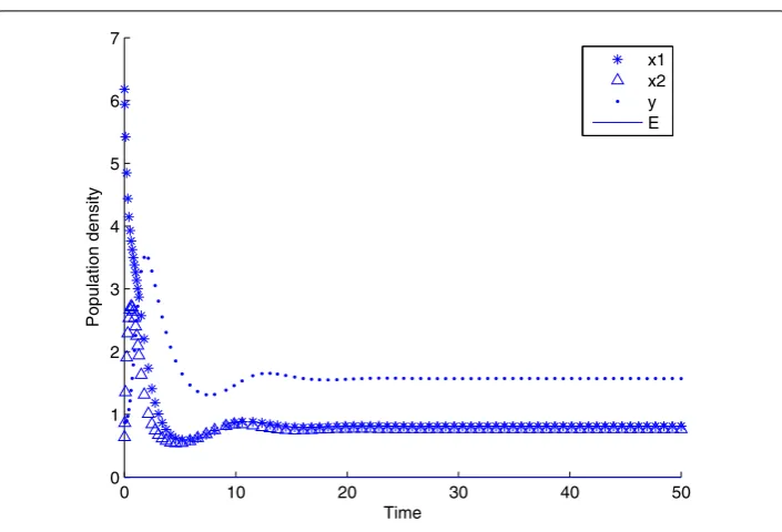
Figure 1 The state response of system (4) withτ= 0.7234 atP3.The state response of system (4) with τ= 0.7234 atP3.

that equation (8) has a positive rootω0= 0.3289, and then the correspondingτ0= 0.7234

can be calculated by solving equation (10). Hence, the interior equilibrium P3 remains

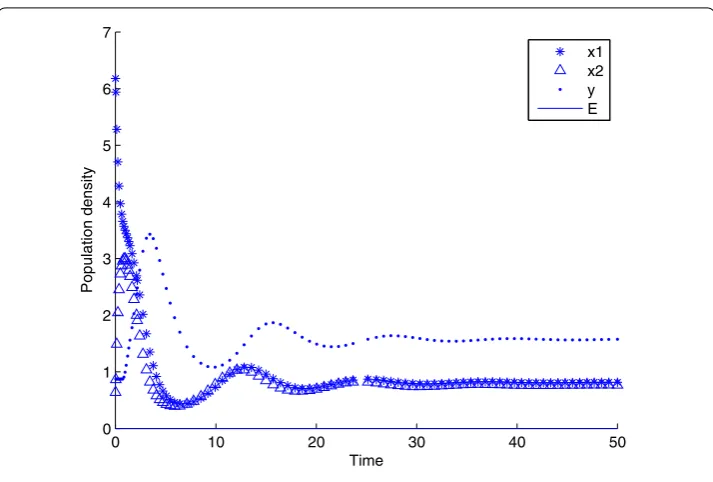
stable forτ< 0.7234. It is shown thatτ= 0.1 in Figure 1 is randomly selected in the interval (0, 0.7234), which is enough to merit the above mathematical study. Asτincreases through

τ0, the phenomenon of Hopf bifurcation occurs forτ0= 0.7234, which is shown in Figure 2.

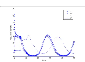
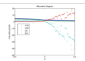
Figure 3 shows a bifurcation diagram of the model forτ0= 0.7234. Figures 4 and 5 show

that system (4) remains unstable for suﬃciently largeτ, but show complex structures with increasing oscillations.

(2) Numerical simulation of the controller.

In order to substantiate the variable structure control theory of above results, the values of parameters are taken as follows:

⎧ ⎪ ⎪ ⎪ ⎪ ⎪ ⎨ ⎪ ⎪ ⎪ ⎪ ⎪ ⎩

dx1(t)

dt = 0.88x2(t) – 0.06x1(t) – 0.56x1(t). dx2(t)

dt = 0.56x1(t) – 0.02x2(t) – 0.1x

2

2(t) – 0.42x2(t)y(t).

dy(t)

dt = 0.42x2(t)y(t) – 0.02y(t) – 0.1y2(t) –E(t)y(t). 0 =E(t)(2.5y(t) – 1.5) –m.

(17)

When the economic profit mvaries, there are some complex dynamic behaviors for model (17) such as the singularity-induced bifurcation. When the economic profitm= 0, model (17) has a positive equilibrium point P∗(6.9951, 4.9284, 0.6, 1.9899). When eco-nomic profitm= –0.02, there are three eigenvalues for the system –0.1677, –1.7101, and –2970.14. The eigenvalues become 2969.53, –0.1677, and –1.7096 when the parameter

m= 0.02. The state response of system (17) is shown in Figure 6 when economic proﬁt

(15)

Figure 2 The state response of system (4) withτ= 0.1 atP3.The state response of system (4) withτ= 0.1

atP3.

Figure 3 The bifurcation diagram of system (4) withτ= 0.7234 atP3.The bifurcation diagram of system

(4) withτ= 0.7234 atP3.

called the over exploitation, and it causes the extinction of the population. Figure 7 shows a bifurcation diagram of the model form= 0.

(16)

Figure 4 The state response of system (4) withτ= 3 atP3.The state response of system (4) withτ= 3

atP3.

Figure 5 The state response of system (4) withτ= 5 atP3.The state response of system (4) withτ= 5

atP3.

population, the adult prey population, the predator population, and harvested eﬀort satisfy the following conditions:

(17)

Figure 6 The state response of system (17) withm= 0.02 atP∗.The state response of system (17) with

m= 0.02 atP∗.

Figure 7 The bifurcation diagram of system (17) withm= 0 atP∗.The bifurcation diagram of system (17) withm= 0 atP∗.

By calculating, we can get the following inequality based on the previous conclusion:

0.2720 <a1< 5.2720, 0 <a0< 2.6460.

(18)

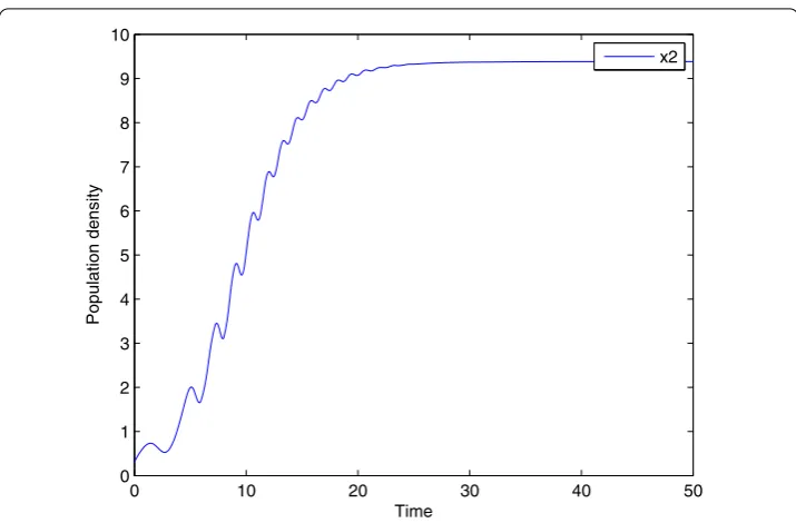
de-Figure 8 Changing of the adult preyx2with variable structure control.Changing of the adult preyx2

with variable structure control.

signed:

η= ⎧ ⎨ ⎩

η+=3|s(e)|10+9.96e2–0.6e1–0.56e2+0.6¯x2

b , s(e) > 0,

η–=–3|s(e)|s(e)|10+9.96e2–0.6e1–0.56e2+0.6¯x2

b , s(e) < 0,

where the sliding surface is deﬁned ass(e) = 9.96e1+e2. In order to illustrate the control

result, numerical simulation is given in Figure 8. In Figure 8, the state variable stays in a stable situation, and the bifurcation behavior is eliminated by the controller. Therefore, variable structure control can stabilize the system eﬀectively.

7 Conclusions

(19)

Acknowledgements

This work was supported by the National Natural Science Foundation of China under Grant No. 61673099, the National Natural Science Foundation of Liaoning Province under Grant No. 2015020007 and Jiangsu Planned Projects for Postdoctoral Research Funds under Grant No. 1401044.

Competing interests

The authors declare that they have no competing interests.

Authors’ contributions

All authors contributed equally and signiﬁcantly in writing this paper. All authors read and approved the ﬁnal manuscript.

Author details

1_{School of Science, Shenyang University of Technology, Shenyang, 110870, China.}2_{School of Automation, Nanjing}

University of Science and Technology, Nanjing, 210094, China.

Publisher’s Note

Springer Nature remains neutral with regard to jurisdictional claims in published maps and institutional aﬃliations.

Received: 20 August 2017 Accepted: 2 December 2017

References

1. Zhang, Q, Liu, C, Zhang, X: Complexity, Analysis and Control of Singular Biological Systems. Springer, London (2012) 2. Niu, H, Zhang, Q: Generalized predictive control for diﬀerence-algebraic biological economic systems. Int. J. Biomath.

6, 1-16 (2013)

3. Jiang, Y, Zhang, Q, Wang, H: Modeling boyciana-ﬁsh-human interaction with partial diﬀerential algebraic equations. Math. Biosci.277, 141-152 (2016)

4. Zhang, Y, Zhang, Q, Li, J: The bifurcation and control of a single-species ﬁsh population logistic model with the invasion of alien species. Discrete Dyn. Nat. Soc.2014, Article ID 548384 (2014). doi:10.1155/2014/548384

5. Zhang, Y, Zhang, Q, Zhang, T:H_∞control of descriptor bioeconomic systems. J. Northeast. Univ.32, 1369-1373 (2011) 6. Zhang, Y, Zhang, Q, Zhao, L: Bifurcation and control in singular biological economic model with stage structure.

J. Syst. Eng.22, 233-238 (2007)

7. Li, L, Zhang, Q, Zhu, B: Fuzzy stochastic optimal guaranteed cost control of bio-economic singular Markovian jump systems. IEEE Trans. Cybern.45, 2512-2521 (2015)

8. Zhang, Y, Zhang, Q, Zhang, G:H_∞control of T-S fuzzy ﬁsh population logistic model with the invasion of alien species. Neurocomputing173, 724-733 (2016)

9. Clark, CW: Mathematical Bioeconomics: The Optimal Management of Renewable Resources. Wiley, New York (1990) 10. Beretta, E, Kuang, Y: Global analyses in some delayed ratio-dependent predator-prey systems. Nonlinear Anal.32,

381-408 (1998)

11. Chakraborty, K, Chakraborty, M, Kar, TK: Bifurcation and control of a bioeconomic model of a prey-predator system with a time delay. Nonlinear Anal. Hybrid Syst.5, 613-625 (2011)

12. Song, Y, Yuan, S: Bifurcation analysis in the delayed Leslie-Gower predator-prey system. Appl. Math. Model.33, 4049-4061 (2009)

13. Yuan, S, Song, Y: Stability and Hopf bifurcations in a delayed Leslie-Gower predator-prey system. J. Math. Anal. Appl.

355, 82-100 (2009)

14. Kar, TK, Ghorai, A: Dynamic behavior of a delayed predator-prey model with harvesting. Appl. Math. Comput.217, 9085-9104 (2011)

15. Martin, A, Ruan, S: Predator-prey models with delay and prey harvesting. J. Math. Biol.43, 247-267 (2001) 16. Emelyanov, SV: Variable Structure Control Systems. Nauka, Moscow (1967)

17. Gao, W, Cheng, M: Variable structure control of ﬂexible spacecraft. J. Beihang Univ.9, 274-280 (1988)

18. Zhang, Q, Li, L, Yan, XG, Spurgeon, SK: Sliding mode control for singular stochastic Markovian jump systems with uncertainties. Automatica79, 27-34 (2017)

19. Venkatasubramanian, V, Schattler, H, Zaborszky, J: Local bifurcations and feasibility regions in diﬀerential-algebraic systems. IEEE Trans. Autom. Control40, 1992-2013 (1995)

20. Freedman, H, Rao, VSH: The trade-oﬀ between mutual interference and time lags in predator-prey systems. Bull. Math. Biol.45, 991-1004 (1983)

21. Erbe, LH, Freedman, H, Rao, VSH: Three-species food-chain models with mutual interference and time delays. Math. Biosci.80, 57-80 (1986)

22. Hale, JK: Theory of Functional Diﬀerential Equations. Springer, New York (1997)

23. Li, J, Zhang, Q, Yan, X, Spurgeon, SK: Integral sliding mode control for Markovian jump T-S fuzzy descriptor systems based on the super-twisting algorithm. IET Control Theory Appl.11, 1134-1143 (2017)