R E S E A R C H
Open Access
A new variable mesh method based on
non-polynomial spline in compression
approximations for 1D quasilinear hyperbolic
equations
Ranjan Kumar Mohanty
1*, Navnit Jha
1and Ravindra Kumar
2,3*Correspondence:
1Department of Applied
Mathematics, South Asian University, Akbar Bhawan, Chanakyapuri, New Delhi, 110021, India
Full list of author information is available at the end of the article
Abstract
In this paper, we present a new three-level implicit method of order two in time and three in space on a non-uniform mesh, based on spline in compression
approximation for the numerical solution of 1D quasilinear second order hyperbolic partial differential equations. We also discuss the application of the proposed method to a wave equation with singular coefficients. Stability analysis of a linear scheme and convergence analysis of a general nonlinear scheme are also discussed in this paper. Computational results are given to demonstrate the usefulness of the proposed method.
MSC: 65M06; 65M12
Keywords: quasilinear hyperbolic equations; variable mesh; spline in compression; non-polynomial spline; wave equation in polar coordinates
1 Introduction
Consider the D quasilinear hyperbolic equation
∂u
∂t =A(x,t,u) ∂u
∂x +f(x,t,u,ux,ut), <x< ,t> . (.)
The initial conditions are given by
u(x, ) =φ(x), ut(x, ) =ψ(x), ≤x≤, (.)
and the boundary conditions are given by
u(,t) =a(t), u(,t) =a(t), t≥. (.)
We assume that the functionsf(x,t,u,ux,ut),φ(x),ψ(x),a(t) anda(t) are sufficiently
smooth and their required higher order derivatives exist.
The wave equations are important second order hyperbolic partial differential equa-tions for the description of waves as they occur in most scientific and engineering dis-ciplines such as sound waves, light waves, water waves, acoustics waves, electromagnetic
waves, and fluid dynamics, optics, electromagnetism, solid mechanics, structural mechan-ics, quantum mechanmechan-ics,etc.The waves for all these applications are described by solu-tions to eitherlinearornonlinearsecond order hyperbolic partial differential equations (.), which have a dependent variableu(x,t) (representing the wave value), an indepen-dent variable timetand one independent spatial variablex. The actual form that the wave takes is strongly dependent upon the system initial conditions, the boundary conditions on the solution domain and any system disturbances. A few examples of the source of physi-cal waves are as follows. Chemiphysi-cal waves occur in the concentration variations of chemiphysi-cal species propagating in a system. Acoustic waves occur in audible sound, medical applica-tions of ultrasound and underwater sonar applicaapplica-tions. Electromagnetic waves occur as electricity in various forms, radio waves, light waves in optic fibres,etc.The transmis-sion of variations in a gravitational field in the form of waves is called gravitational waves as predicted by Einstein’s theory of general relativity. Waves resulting from earthquakes, large explosions and high velocity impacts are termed seismic waves. Small local changes in velocity occurring in high density situations can result in the propagation of traffic flow waves and even shocks. When ripples occur in water, they are manifested as waves of short length and are termed capillary waves. For waves where the wavelength is much greater than water depth, they can be modelled by coupled fluid dynamics equations known as the shallow water wave equations.
Nonlinear waves are described by nonlinear equations. This means that nonlinear wave equations are more difficult to analyze mathematically and that no general analytical method for their solution exists. Hence the only alternative to solve these equations is the application of stable numerical methods. In this paper, using three non-uniform grid points inx-direction and three uniform grid points int-direction, we discuss a new three-level implicit method of accuracy two in time and three in space based on spline in com-pression approximations for the solution of D second order quasilinear hyperbolic equa-tions. In this method, we require only three evaluations of functionf. In Section , we discuss spline in compression and its properties. In Section , we propose a new three-level implicit method based on spline in compression approximation. In Section , we derive the proposed method. In Section , we discuss the application of our method to the wave equation in polar cylindrical coordinates. Stability and convergence analysis are discussed in Sections and . In Section , we discuss the higher order approximation at first time level in order to compute the proposed numerical method of the same accuracy and compare the numerical results with the existing results. Final remarks are given in Section .
2 Spline in compression approximation
The solution domain [, ]×[t> ] is divided into (N+ )×Jvariable mesh with the variable spatial step sizehl=xl–xl–,l= , , . . . ,N+ , inx-direction and the time step size k> int-direction, whereNis a positive integer. Grid points are given byxl=x+
l i=hi, l= , , . . . ,N+ , andtj=jk,j= , , , . . . . The mesh ratio parameter is given byσl=hl+/hl, l= , , . . . ,N. The notationsujlandUljare used for the discrete approximation and the exact value ofu(x,t) at the grid point (xl,tj), respectively. Similarly, at the grid point (xl,tj),
we defineAjl=A(xl,tj),Axjl=Ax(xl,tj), . . . ,etc.
LetSj(x) be the non-polynomial spline in compression of the functionu(x,t) at the grid
point (xl,tj) and be given by
Sj(x) =al+bl(x–xl) +clsinω(x–xl) +dlcosω(x–xl), l= , , , . . . ,N+ , (.)
whereal,bl,cl,dlare unknown coefficients andωis a parameter to be determined.Sj(x)∈ C[, ], which interpolatesu(x,t) at the grid point (x
l,tj).
The derivatives of functionSj(x) are given by
Sj(x) =bl+ωclcosω(x–xl) –ωdlsinω(x–xl),
l= , , , . . . ,N+ ;j= , , . . . ,J, (.)
Sj(x) = –ωclsinω(x–xl) +dlcosω(x–xl)
,
l= , , , . . . ,N+ ;j= , , . . . ,J. (.)
We define
Mjl=Sj(xl), l= , , , . . . ,N+ ;j= , , . . . ,J. (.)
To derive expression for the coefficients of (.) in terms ofUlj,Ul+j ,MljandMjl+, we use
Sj(xl) =Ulj, Sj(xl+) =Ul+j , M j
From algebraic manipulation, we get
to the cubic spline relation on the variable mesh
Ul+j –Ulj
alent to the equationtanθl
=
θl
. This equation has an infinite number of roots. Solving
graphically, we obtain the smallest nonzero positive valueθl= ..
Further, using the relationsθl=ωhl,θl+=ωhl+, from (.) and (.), we have
Note that (.), (.), (.) and (.) are important properties of the spline in a com-pression functionSj(x).
3 Variable mesh method based on spline in compression approximation
For the sake of simplicity, we chooseσl=hl+/hl=σ (a constant), that is,hl+=σhl, and
we consider the one-space dimensional nonlinear hyperbolic partial differential equation
∂u
∂t =A(x,t) ∂u
∂x +f(x,t,u,ux,ut), <x< ,t> (.)
with the given initial conditions (.) and boundary conditions (.). Now, we consider the following approximations:
Since the derivative values ofSj(x) defined by (.)-(.) are not known at each grid
Now we define the approximations
ˆ
l), approximation of its first order
space derivative defined by (.)-(.) inx-direction and central difference approximations of time derivative defined by (.)-(.) int-direction.
Then, at each grid point (xl,tj), the differential equation (.) is discretized by
4 Mathematical derivation of the method
For the derivation of method (.), we use spline in compression approximations in x-direction and second order finite difference approximation int-direction.
At the grid point (xl,tj), let us denote
Using the Taylor expansion, we obtain
Simplifying (.)-(.), we get
Ut
With the help of approximations (.) and (.), from (.), we obtain
Similarly,
Now using approximations (.)-(.) in (.)-(.) and simplifying (.)-(.), we get
Now we define the approximation
ˆ
where ‘a’ and ‘b’ are parameters to be determined. By the help of approximations (.), (.), (.), (.) and (.), from (.) we obtain
for the values of parametersa= α
(+σ)Ajl andb=
αAxjl
Ajl , approximation (.) reduces to
ˆ
mjl=mjl+Ok+khl+hl
. (.)
Now, with the help of approximations (.) and (.), from (.), we obtain
ˆ
Using approximations (.)-(.) and (.)-(.), from (.) and (.), we obtain the local truncation errorTˆlj=O(kh
l +khl +hl).
Now, we consider the numerical method ofO(k+kh
l+hl) for the solution of
quasi-linear hyperbolic equation (.).
values:
Axjl=
σ( +σ)hl
Ajl+– –σAjl–σAjl–+Ohl, (.)
Axxjl=
σ( +σ)h l
Ajl+– ( +σ)Ajl+σAjl–+O(hl), (.)
where
Ajl=Axl,tj,Ulj
,
Ajl±=Axl±,tj,Ulj±
.
Thus, substituting values (.)-(.) into (.), we obtain the required numerical method ofO(k+kh
l+hl) for the solution of the quasilinear hyperbolic equation (.),
and hence the local truncation error retains its order, that is,Tˆlj=O(khl+khl+hl). For hl+=hl=h, the proposed method (.) becomes ofO(k+kh+h) (see []).
Note that the initial and Dirichlet boundary conditions are given by (.) and (.), re-spectively. Incorporating the initial and boundary conditions, we can write method (.) in a tri-diagonal matrix form. If the differential equation (.) is linear, we can solve the linear system using the Gauss-elimination (tri-diagonal solver) method; in the nonlinear case, we can use the Newton-Raphson iterative method to solve the nonlinear system (see Kelly [], Hageman and Young []).
5 Application to a wave equation in polar coordinates
We consider the one-space dimensional wave equation in polar coordinates
utt=urr+D(r)ur+f(r,t), <r< ,t> . (.)
The initial and the Dirichlet boundary conditions are prescribed by
u(r, ) =φ(r), ut(r, ) =ψ(r), ≤r≤, (.)
u(,t) =q(t), u(,t) =q(t), t≥, (.)
whereD(r) =γr. Forγ = and , equation (.) represents a wave equation in cylindrical and spherical polar coordinates, respectively. Assume thatf(r,t)∈C(, )×[t> ] and conditions (.) and (.) are given with sufficient smoothness to maintain the order of accuracy in the numerical method under consideration.
Replacing the variablexbyr, applying method (.) to (.) and neglecting the local truncation error, we obtain
h l
ujl+– ( +σ)ujl+σujl–
=Puttjl+–Dl+uˆrjl+–f j l+
+Quttjl–Dluˆrjl–f j l
+Ruttjl––Dl–uˆrjl––f j l–
where
where the approximations associated with (.) are defined in Section . Note that scheme (.) is ofO(k+kh
l+hl) accuracy for the solution of wave equation
(.). Sincer= , scheme (.) fails to compute atl= due to zero division. In order to
–PD
Note that the numerical scheme (.) based on spline in compression approximations is ofO(k+kh
l+hl) accuracy and free from the terms /(rl±), hence very easily solved
forl= ()N in the solution region <r< ,t> . This technique shows that the pro-posed method is applicable to singular problems, and we do not require the presence of any fictitious points outside the solution region to handle the numerical scheme near the boundary.
6 Stability analysis
Consider the damped wave equation in a general form
wtt+ ηwt=wxx+f(x,t), <x< ,t> , (.)
whereη> is a real parameter.
The damped wave equation is a linear second order hyperbolic partial differential equa-tion. The term ηwtrepresents a damping force proportional to the velocitywt.
Replacing the variableubywand applying scheme (.) to the differential equation (.) withη= , that is,hl+=hl=h, we obtain a numerical approximation ofO(k+h) as
The corresponding error equation is
To establish stability for scheme (.), it is necessary to assume that the solution of the homogeneous part of the error equation (.) is of the formεjl=ξjeiθl, wherei=√–,θ
is real, and we obtain the characteristic equation
The necessary and sufficient condition for|ξ|< is thatp+q+r> ,p–r> ,p–q+r> .
In order to obtain an unconditionally stable spline in compression finite difference scheme ofO(k+h) accuracy, we may re-write scheme (.) as order and does not affect the consistency and accuracy of the scheme. Like (.), the char-acteristic equation for (.) may be written as
p∗ξ+q∗ξ+r∗= , (.)
Thus, for stability, we must have the conditions
(i) p∗+q∗+r∗= λsin
We can treat this separately:
(ii) p∗–r∗=ηk
We treat this case separately. Forθ= or π, we have the characteristic equation
( +ηk)ξ– ξ+ ( –ηk) = (.)
whose roots areξ,= ,–+ηηkk. In this case also|ξ| ≤.
7 Convergence analysis
We consider the nonlinear hyperbolic differential equation
∂w ∂t =
∂w
∂x +g(x,t,w,wx,wt), <x< ,t> . (.)
The initial and boundary conditions are given by
w(x, ) =a(x), wt(x, ) =b(x), ≤x≤, (.)
w(,t) =a(t), w(,t) =a(t), t≥. (.)
In this section, we establish under appropriate conditions the fourth order convergence of the proposed method.
We assume that the initial value problem (.)-(.) has a unique smooth solutionw(x,t), and the following conditions (see []) are satisfied:
(i) g(x,t,w,wx,wt)is continuous,
(ii) g(x,t,w,wx,wt)satisfies the Lipschitz condition, namely g(x,t,w+ξ,wx+ξ,wt+ξ) –g
x,t,w+ξ∗,wx+ξ∗,wt+ξ∗
≤L ξ–ξ∗ + ξ–ξ∗ + ξ–ξ∗ ,
whereξiandξi∗are arbitrary real numbers, andLis a Lipschitz constant, (iii) a(x)andb(x)are continuously differentiable up to order and , respectively.
Forhl+=hl=h,λ= (k/h) > and replacing the variablesUbyW,ubyw, we may re-write
scheme (.) as
λWl+j – Wlj+Wl–j –kW tt
j l++Wtt
j
l–+ Wtt j l
+kGˆjl++Gˆjl–+ Gˆjl=Tlj, l= ()N;j= , , , . . . , (.) where
Gjl=gxl,tj,Wlj,Wx j l,Wt
j l
, Gˆjl=gxl,tj,Wlj,Wˆxjl,Wt j l
, etc., . . . and
Tlj=Ok+kh+kh.
Let Wj= [Wj,W j , . . . ,W
j
N]T(Tdenotes transpose) and wj= [w j ,w
j , . . . ,w
j
N]Tbe the
ex-act and approximate solution vectors of the solutionw(x,t) at the grid point (xl,tj),
respec-tively, and let T = [Tj,Tj, . . . ,TNj]Tbe the local truncation error vector.
Let
φ(W)≡φWj+, Wj, Wj–=kGˆl+j +Gˆjl–+ Gˆjl
and
φ(w)≡φwj+, wj, wj–=kgˆl+j +gˆl–j + gˆjl,
where
gjl=gxl,tj,wjl,wxjl,wtjl
, gˆjl=gxl,tj,wjl,wˆxjl,wtjl
Then the spline in compression method described by (.) can be expressed in a matrix form as follows:
DWj++ CWj+ DWj–+φ(W) = T, (.)
where D = [–, –, –]Tand C = [ + λ, – λ, + λ]Tare tri-diagonal matrices of orderN.
The method consists of obtaining an approximation wj+ for Wj+ by solving the tri-diagonal system
Further, we may write
With the help of (.c) and (.d), we obtain
φ(w) –φ(W) = PEj++ QEj+ REj–, (.)
where P, Q and R are the coefficient matrices of error vectors Ej+, Ejand Ej–, respectively.
Subtracting (.) from (.), we have
(D + P)Ej++ (C + Q)Ej+ (D + R)Ej–= –T. (.)
Assume that the exact solution values ofw(x,t) are known exactly at initial and first time levels so that Ej= Ej–= . Then from (.) we obtain the error equation
(D + P)Ej+= –T. (.)
LetPl,mbe the (l,m)th element of matrix P, then it is easy to verify that
– +Pl,l±< forl= ()N– , ()N,
and hence D + P is irreducible (see Varga []).
LetSmbe the sum of the elements of themth row of D + P andI∗=Min[(α–β)Ilj·J j xl–
(α+βJlj)Ixjl], then, for sufficiently smallhandk, we obtain
Sm> khI∗
, m= andN, (.a)
Sm≥khI∗, m= ()N– (.b)
and hence D + P is also monotone.
Then (D + P)–exists (D + P)–≥ (see Varga []).
Since
N
m=
(D + P)–l,m·Sm= , l= ()N,
hence
(D + P)–l,m≤ Sm ≤
khI∗, l= ()N;m= andN (.a)
and
N
m=
(D + P)–l,m≤
MinSm ≤
khI∗, l= ()N. (.b)
From (.), we have
Now,
εj+l ≤(D + P)–l,|T|+ N–
m=
(D + P)–l,m· |Tm|+ (D + P)–l,N|TN|, l= ()N. (.)
LetEj+=max{|εj+
l |:l= ()N}.
With the help of (.a) and (.b) and whenk∝h, from (.), we obtain, for
suffi-ciently smallhandk,
Ej+=Oh. (.)
This establishes the fourth order convergence of the method.
8 Numerical results
Substituting approximations (.), (.), (.) and (.) directly into the differential equa-tion (.), we obtain a method
Utt j l=A
j lUxx
j l+f
xl,tj,Ulj,Ux j l,Ut
j l
+Ok+hl
, l= ()N,j= , , . . . . (.)
In this section, we solve some benchmark problems using the method described by equa-tion (.) and compare our results with the results obtained by using the method dis-cussed in []. The exact solutions are provided in each case. The right-hand side ho-mogeneous functions, initial and boundary conditions may be obtained using the exact solution as a test procedure. The linear difference equations have been solved using a direct method, that is, tri-diagonal solver; whereas nonlinear difference equations have been solved using the Newton-Raphson iteration method. For the Newton-Raphson it-eration method, we have chosen zero vector as the initial guess and the itit-erations were stopped when the error tolerance ≤– was achieved. All computations were
car-ried out using double precision arithmetic. All computations were done using MATLAB codes. Throughout computation, we have used ωl =ωl+ =ω. From consistency
con-dition, we found the relation tan(ωhl
) =
ωhl
. This equation has an infinite number of
roots, the smallest positive nonzero root being given byωhl= .. We have used ωhl= . (fixed) throughout the computation, that is,ω= (.)/hl. For
different values of ‘hl’, we have different values of ‘ω’. That would not affect the accuracy
of the scheme.
Note that the proposed method (.) for second order quasilinear hyperbolic equations is a three-level scheme. The value ofuatt= is known from the initial condition. To start any computation, it is necessary to know the numerical value ofuof required accuracy at t=k. In this section, we discuss an explicit scheme ofO(k) foruat first time level, i.e., att=kin order to solve the differential equation (.) using method (.), which is applicable to problems in Cartesian and polar coordinates.
Since the values ofuandutare known explicitly att= , this implies that all their
suc-cessive tangential derivatives are known att= ,i.e., the values ofu,ux,uxx, . . . ,ut,utx, . . . , etc.are known att= .
An approximation foruofO(k) att=kmay be written as
ul =ul +kutl + k
(utt)
l +O
From equation (.), we have
(utt)l =
A(x,t,u)uxx+f(x,t,u,ux,ut)
l. (.)
Thus, using the initial values and their successive tangential derivative values, from (.) we can obtain the value of (utt)l, and then, ultimately, from (.) we can compute the value
ofuat first time level,i.e., att=k. Replacing the variablexbyrin (.), we can also obtain an approximation ofO(k) foruatt=kfor problems in polar coordinates.
We discretize the solution domain={(x,t)| <x< ,t> }such that =x<x<· · ·< xN <xN+= , wherehl=xl–xl–andσ=hl+/hl> ,l= ()N,
=xN+–x=xN+–xN+xN–xN–+· · ·+x–x
=hN++hN+hN–+· · ·+h
= +σ+σ+· · ·+σNh. (.)
Thus
h=
–σ
–σN+, σ= . (.)
Hence, by prescribing the total number of mesh pointsN+ , we can compute the value ofhfrom (.). The remaining mesh is determined byhl+=σhl,l= , , . . . ,N. We have
chosenσ= .. We have takenN+ = , , , as the total number of grid points in thex-direction. Therefore, to obtain the numerical solution att= ., we choose the time stepk= ./(N+ ).
Example (Wave equation in polar coordinates)
∂u ∂t =
∂u ∂r +
γ r
∂u
∂r+f(r,t), <r< ,t> . (.)
The initial and boundary conditions are given by
u(r, ) = , ut(r, ) =coshr, ≤r≤, (.)
u(,t) =sint, u(,t) =coshsint, t≥. (.)
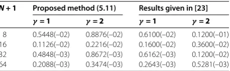
The exact solution is given byu(r,t) =coshrsinht. The maximum absolute errors (MAE) are tabulated in Table att= . forγ = and .
Table 1 Example 1: the maximum absolute errors
N + 1 Proposed method (5.11) Results given in [23]
γ= 1 γ= 2 γ= 1 γ= 2
Table 2 Example 2: the maximum absolute errors
N + 1 Proposed method (3.20) Results given in [23]
γ= 1 γ= 2 γ= 3 γ= 1 γ= 2 γ= 3
8 0.1615(–04) 0.1211(–04) 0.1132(–04) 0.2676(–04) 0.1610(–04) 0.1473(–04) 16 0.1433(–05) 0.1008(–05) 0.8878(–06) 0.2138(–05) 0.1210(–05) 0.9764(–06) 32 0.1515(–06) 0.1068(–06) 0.6704(–07) 0.2363(–06) 0.1236(–06) 0.7923(–07) 64 0.1688(–07) 0.1082(–07) 0.5315(–08) 0.2665(–07) 0.1332(–07) 0.6733(–08)
Table 3 Example 3: the maximum absolute errors
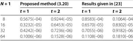
N + 1 Proposed method (3.20) Results given in [23]
t = 1 t = 2 t = 1 t = 2
8 0.5675(–04) 0.9244(–05) 0.8583(–04) 0.1064(–04) 16 0.3232(–05) 0.6453(–05) 0.6570(–05) 0.8302(–05) 32 0.4242(–06) 0.7236(–06) 0.7055(–06) 0.9182(–06) 64 0.1006(–06) 0.1528(–06) 0.1108(–06) 0.1810(–06)
Example (Van der Pol type nonlinear wave equation)
∂u ∂t =
∂u ∂x +γ
u– ∂u
∂t +f(x,t), <x< ,t> . (.)
The initial and boundary conditions are given by
u(x, ) =sinπx, ut(x, ) = –γsinπx, ≤x≤, (.)
u(,t) =sint, u(,t) =coshsint, t≥. (.)
The exact solution is given byu(x,t) =e–γtsinπx. The MAE are tabulated in Table at t= . forγ = , and .
Example (Dissipative nonlinear wave equation)
∂u ∂t =
∂u ∂x – u
∂u
∂t +f(x,t), <x< ,t> . (.)
The initial and boundary conditions are given by
u(x, ) = , ut(x, ) =sinπx, ≤x≤, (.)
u(,t) = , u(,t) = , t≥. (.)
The exact solution is given byu(x,t) =sinπxsint. The MAE are tabulated in Table at t= and .
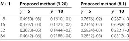
Example (Quasi-linear hyperbolic equation)
∂u ∂t =
+x+u∂ u
∂x +γu
∂u ∂x+
∂u ∂t
Table 4 Example 4: the maximum absolute errors
N + 1 Proposed method (3.20) Proposed method (8.1)
γ= 5 γ= 10 γ= 5 γ= 10
8 0.4950(–03) 0.1610(–01) 0.7676(–02) 0.2871(–00) 16 0.3597(–04) 0.1421(–02) 0.2346(–02) 0.6952(–01) 32 0.3023(–05) 0.1444(–03) 0.6924(–03) 0.2221(–01) 64 0.4042(–06) 0.2188(–04) 0.2852(–03) 0.8512(–02)
The initial and the boundary conditions are given by
u(x, ) =coshx, ut(x, ) =coshx, ≤x≤, (.)
u(,t) =et, u(,t) =etcosh, t≥. (.)
The exact solution is given by u=etcoshx. The MAE are tabulated in Table forγ =
and att= .
9 Final remarks
Available numerical methods based on spline in compression approximations for the nu-merical solution of second order quasilinear hyperbolic equations on a variable mesh are ofO(k+h
l) accuracy only. In this article, using the same number of grid points and three
evaluations of the functionF, we have derived a new stable method ofO(k+kh l+hl)
accuracy for the solution of second order quasilinear hyperbolic equation (.). To demon-strate the efficiency and the applicability of the proposed method, we have applied it to a few benchmark problems and have obtained convergent results. The results were com-pared with the results obtained by using a Numerov type method discussed in [], and they show superiority over the latter. The non-polynomial basis{,x,sinx,cosx}consists ofC∞-differentiable functions, which compensates the loss of smoothness inherited by standard Numerov type discretization discussed in []. Therefore, the numerical method (.) based on non-polynomial spline approximations gives better results compared with the results given in [].
Competing interests
The authors declare that they have no competing interest.
Authors’ contributions
RKM discussed the variable mesh method based on spline in compression approximation and stability analysis. NJ discussed the convergence analysis and the application of the proposed method to singular problems. RK carried out all the computational work. All authors read and approved the final manuscript.
Author details
1Department of Applied Mathematics, South Asian University, Akbar Bhawan, Chanakyapuri, New Delhi, 110021, India. 2Department of Mathematics, Faculty of Mathematical Sciences, University of Delhi, Delhi, 110007, India.3Department of
Mathematics, Rajdhani College, University of Delhi, New Delhi, 110015, India.
Acknowledgements
The authors thank the reviewers for their valuable suggestions which substantially improved the standard of the paper.
Received: 14 April 2015 Accepted: 14 October 2015
References
1. Bickley, WG: Piecewise cubic interpolation and two point boundary value problems. Comput. J.11, 206-208 (1968) 2. Fyfe, DJ: The use of cubic splines in the solution of two point boundary value problems. Comput. J.12, 188-192
3. Fleck, JA Jr.: A cubic spline method for solving the wave equation of nonlinear optics. J. Comput. Phys.16, 324-341 (1974)
4. Raggett, GF, Wilson, PD: A fully implicit finite difference approximation to the one-dimensional wave equation using a cubic spline technique. J. Inst. Math. Appl.14, 75-77 (1974)
5. Jain, MK, Aziz, T: Spline function approximation for differential equations. Comput. Methods Appl. Mech. Eng.26, 129-143 (1981)
6. Jain, MK, Aziz, T: Cubic spline solution of two-point boundary value problems with significant first derivatives. Comput. Methods Appl. Mech. Eng.39, 83-91 (1983)
7. Al-Said, EA: Spline methods for solving a system of second order boundary value problems. Int. J. Comput. Math.70, 717-727 (1999)
8. Kadalbajoo, MK, Bawa, RK: Cubic spline method for a class of non-linear singularly perturbed boundary value problems. J. Optim. Theory Appl.76, 415-428 (1993)
9. Al-Said, EA: The use of cubic splines in the numerical solution of a system of second order boundary value problem. Comput. Math. Appl.42, 861-869 (2001)
10. Aziz, T, Khan, A: A spline method for second-order singularly perturbed boundary value problems. J. Comput. Appl. Math.147, 445-452 (2002)
11. Jain, MK, Iyengar, SRK, Pillai, ACR: Difference schemes based on splines in compression for the solution of conservation laws. Comput. Methods Appl. Mech. Eng.38, 137-151 (1983)
12. Kadalbajoo, MK, Patidar, KC: Numerical solution of singularly perturbed non-linear two point boundary value problems by spline in compression. Int. J. Comput. Math.79, 271-288 (2002)
13. Kadalbajoo, MK, Patidar, KC: Variable mesh spline in compression for the numerical solution of singular perturbation problems. Int. J. Comput. Math.80, 83-93 (2003)
14. Kadalbajoo, MK, Aggarwal, VK: Cubic spline for solving singular two-point boundary value problems. Appl. Math. Comput.156, 249-259 (2004)
15. Talwar, J, Mohanty, RK: Spline in compression method for non-linear two point boundary value problems on a geometric mesh. Neural Parallel Sci. Comput.21, 553-570 (2013)
16. Mohanty, RK, Jha, N, Evans, DJ: Spline in compression method for the numerical solution of singularly perturbed two point singular boundary value problems. Int. J. Comput. Math.81, 615-627 (2004)
17. Mohanty, RK, Jha, N: A class of variable mesh spline in compression methods for singularly perturbed two point singular boundary value problems. Appl. Math. Comput.168, 704-716 (2005)
18. Tirmizi, IA, Haq, FI, Islam, SU: Non-polynomial spline solution of singularly perturbed boundary-value problems. Appl. Math. Comput.196, 6-16 (2008)
19. Mohanty, RK, Jain, MK, George, K: On the use of high order difference methods for the system of one space second order non-linear hyperbolic equations with variable coefficients. J. Comput. Appl. Math.72, 421-431 (1996) 20. Mohanty, RK, Arora, U: A new discretization method of order four for the numerical solution of one space
dimensional second order quasi-linear hyperbolic equation. Int. J. Math. Educ. Sci. Technol.33, 829-838 (2002) 21. Mohanty, RK, Singh, S: High accuracy Numerov type discretization for the solution of one-space dimensional
non-linear wave equations with variable coefficients. J. Adv. Res. Sci. Comput.3, 53-66 (2011)
22. Mohanty, RK, Gopal, V: An off-step discretization for the solution of 1D mildly nonlinear wave equations with variable coefficients. J. Adv. Res. Sci. Comput.4, 1-13 (2012)
23. Mohanty, RK, Singh, S: High order variable mesh approximation for the solution of 1D non-linear hyperbolic equation. Int. J. Nonlinear Sci.14, 220-227 (2012)
24. Mohanty, RK, Kumar, R: A new fast algorithm based on half-step discretization for one space dimensional quasilinear hyperbolic equations. Appl. Math. Comput.244, 624-641 (2014)
25. Rashidinia, J, Jalilian, R, Kazemi, V: Spline methods for the solutions of hyperbolic equations. Appl. Math. Comput.190, 882-886 (2007)
26. Ding, H, Zhang, Y: Parametric spline methods for the solution of hyperbolic equations. Appl. Math. Comput.204, 938-941 (2008)
27. Mohanty, RK: An unconditionally stable difference scheme for the one space dimensional linear hyperbolic equation. Appl. Math. Lett.17, 101-105 (2004)
28. Mohanty, RK: New unconditionally stable difference schemes for the solution of multi-dimensional telegraphic equations. Int. J. Comput. Math.86, 2061-2071 (2009)
29. Ding, H, Zhang, Y: A new unconditionally stable compact difference scheme ofO(τ2+h4) for the 1D linear
hyperbolic equation. Appl. Math. Comput.207, 236-241 (2009)
30. Ding, H, Zhang, Y, Cao, J, Tian, J: A class of difference scheme for solving telegraph equation by new non-polynomial spline methods. Appl. Math. Comput.218, 4671-4683 (2012)
31. Mohanty, RK, Gopal, V: High accuracy cubic spline finite difference approximation for the solution of one-space dimensional non-linear wave equations. Appl. Math. Comput.218, 4234-4244 (2011)
32. Mohanty, RK, Dahiya, V, Khosla, N: Spline in compression methods for singularly perturbed 1D parabolic equations with singular coefficients. J. Discrete Math.2, 70-77 (2012)
33. Talwar, J, Mohanty, RK, Singh, S: A new spline in compression approximation for one space dimensional quasilinear parabolic equations on a variable mesh. Appl. Math. Comput.260, 82-96 (2015)
34. Gopal, V, Mohanty, RK, Jha, N: New non-polynomial spline in compression method ofO(k2+h4) for the solution of 1D
wave equation in polar co-ordinates. Adv. Numer. Anal.2013, Article ID 470480 (2013)
35. Mohanty, RK, Gopal, V: High accuracy non-polynomial spline in compression method for one-space dimensional quasi-linear hyperbolic equations with significant first order space derivative term. Appl. Math. Comput.238, 250-265 (2014)
36. Kelly, CT: Iterative Methods for Linear and Nonlinear Equations. SIAM, Philadelphia (1995) 37. Hageman, LA, Young, DM: Applied Iterative Methods. Dover, New York (2004)
38. Li, WD, Sun, ZZ, Zhao, L: An analysis for a high order difference scheme for numerical solution to