R E S E A R C H
Open Access
Necessary and sufficient condition for
existence of periodic solutions of
predator-prey dynamic systems with
Beddington-DeAngelis-type
functional response
Neslihan Nesliye Pelen
1*, A. Feza Güvenilir
2and Billur Kaymakçalan
3*Correspondence:
nesliyeaykir@gmail.com 1Department of Mathematics,
Ondokuz Mayıs University, Samsun, Turkey
Full list of author information is available at the end of the article
Abstract
We consider two-dimensional predator-prey systems with
Beddington-DeAngelis-type functional response on periodic time scales. For this special case, we try to find the necessary and sufficient conditions for the considered system when it has at least onew-periodic solution. This study is mainly based on continuation theorem in coincidence degree theory and will also give beneficial results for continuous and discrete cases. Especially, for the continuous case, by using the study of Cui and Takeuchi (J. Math. Anal. Appl. 317:464-474, 2006), to obtain the globally attractivew-periodic solution of the given system, an inequality is given as a necessary and sufficient condition. Additionally, for the continuous case in this study, the open problem given in the discussion part of the study of Fan and Kuang (J. Math. Anal. Appl. 295:15-39, 2004) is solved.
Keywords: predator-prey dynamic systems; Beddington-DeAngelis-type functional response; continuation theorem; globally attractive solution; periodic solution; time-scale calculus
1 Introduction
The relationships between species and the outer environment and the connections be-tween different species are the description of the predator-prey dynamic systems, which are the subject of mathematical ecology in biomathematics. Various types of functional re-sponses in a predator-prey dynamic system such as Monod-type, semi-ratio-dependent, and Holling-type have been studied in [–].
The key concepts in this study are the functional response in the periodic environment and the time-scale calculus.
First of all, we investigate the predator-prey system with Beddington-DeAngelis-type functional response for a general time scale and its continuous case. This type of func-tional response first appeared in [] and []. At low densities, with this type of funcfunc-tional response, some of the singular behaviors of ratio-dependent models are avoided. Also,
predator feeding can be described much better over a range of predator-prey abundances by using Beddington-DeAngelis-type functional response.
Secondly, being in a periodic environment is important because, in such an environ-ment, the global existence and stability of a positive periodic solution is a significant prob-lem in population growth model. This plays a similar role as a globally stable equilibrium in an autonomous model. Therefore, it is important to consider under which conditions the resulting periodic nonautonomous system would have a positive periodic solution that is globally asymptotically stable, and the globally asymptotically stable periodic solution of the given system in the continuous case is investigated in this study as an application. For nonautonomous case, there are many studies on the existence of periodic solutions of predator-prey systems in continuous and discrete models based on the coincidence theory such as [, –].
Additionally, for the continuous case, the studies of Fan and Kuang [] and Cui and Takeuchi [] have very important contributions on the predator-prey dynamic systems with Beddington-DeAngelis-type functional response. They have investigated the follow-ing equation:
˜
x(t) =a(t)˜x(t) –b(t)˜x(t) – c(t)˜y(t)˜x(t) α(t) +β(t)˜x(t) +m(t)˜y(t),
˜
y(t) = –d(t)y˜(t) + f(t)˜x(t)˜y(t) α(t) +β(t)˜x(t) +m(t)˜y(t).
()
Here x˜ andy˜ represent the densities of the populations of the prey and predator. In other words, they represent the numbers of individuals in the prey and predator popula-tion per unit area, respectively. For general nonautonomous case, Fan and Kuang studied the permanence, extinction, and global asymptotic stability of the given system. For the periodic case, Fan and Kuang established two sufficient criteria for the existence of a posi-tive periodic solution by using Brouwer fixed point theorem and continuation theorem in coincidence degree theory, respectively. These criteria are easy to be verified for the given system in the form of (). At the same time, authors pointed that these criteria have room for further improvement. They presented numerical simulation to indicate that () may admit positive periodic solutions when the conditions in the theorems fail.
On the basis of these obtained results for system () with periodic coefficients, Cui and Takeuchi continue the study on the periodic solution and permanence of that system. Cui and Takeuchi obtained some new conditions for the permanence and existence of a pos-itive periodic solution of system (). These results improve those obtained by Fan and Kuang []. In addition to this improvement, in their paper [], they also give the equiv-alence between the permanence and satisfaction of the inequality in Theorem . in []. However, they could not show whether there is the equivalence between the existence of at least onew-periodic solution and satisfaction of the inequality in Theorem . in [].
solution. Therefore, we are able to show that to obtain a periodic solution for the periodic case of system (), the improvement of this inequality becomes impossible.
Thirdly, the unification of continuous and discrete analysis is also significant for this study. To unify the study of differential and difference equations, the theory of time-scale calculus is initiated by Stephan Hilger []. In [, ] unification of the existence of periodic solutions of population models modeled by ordinary differential equations and their dis-crete analogues in the form of difference equations and extension of these results to more general time scales is studied. The aim of this study is to find a necessary and sufficient condition for the periodic solution of the given system with Beddington-DeAngelis-type functional response for a general time scale and apply this result to the continuous case.
In this paper, we investigate the system
x(t) =a(t) –b(t)expx(t)– c(t)exp(y(t))
α(t) +β(t)exp(x(t)) +m(t)exp(y(t)),
y(t) = –d(t) + f(t)exp(x(t))
α(t) +β(t)exp(x(t)) +m(t)exp(y(t)).
()
HereTis periodic, that is, ift∈Tthent+w∈T, anda(t),b(t),c(t),d(t),f(t),α(t),β(t),m(t) arew-periodic functions inT. We definew-periodic functionsh(t) inTbyh(t+w) =h(t). All the coefficient functions are positive. This system on time scales was studied in [, –].
2 Preliminaries
The necessary information is taken from []. Let X, Z be normed vector spaces, L: DomL⊂X→Zbe a linear mapping, andN:X→Zbe a continuous mapping. The
map-pingLwill is called a Fredholm mapping of index zero ifdim KerL=codim ImL< +∞and ImLis closed inZ. IfLis a Fredholm mapping of index zero and there exist continuous
projectionsP:X→XandQ:Z→Zsuch thatImP=KerLandImL=KerQ=Im(I–Q), then it follows thatL|DomL∩KerP: (I–P)X→ImLis invertible. We denote the inverse of
that map byKP. Ifis an open bounded subset ofX, then the mappingN is calledL
-compact onifQN() is bounded andKP(I–Q)N:→Xis compact. SinceImQis
isomorphic toKerL, there exists an isomorphismJ:ImQ→KerL.
Definition ([]) The codimension (or quotient or factor dimension) of a subspaceLof a vector spaceV is the dimension of the quotient spaceV/L; it is denoted bycodimVLor
simply bycodimLand is equal to the dimension of the orthogonal complement ofLinV, and we havedimL+codimL=dimV.
The given information is necessary for the following continuation theorem.
Theorem ([], continuation theorem) Let L be a Fredholm mapping of index zero,and N be L-compact on.Let the following conditions be satisfied:
(a) For eachλ∈(, ),every solutionzofLz=λNzis such thatz∈/δ; (b) QNz= for eachz∈δ∩KerL,and the Brouwer degree
deg{JQN,δ∩KerL, } = .
Definition ([]) A subsetA⊂Crd(X,R) is said to be rd-equicontinuous if the following
items are satisfied:
• For all right dense points oft∈Xand for each> , there existsδ> such that for
allt∈T, we have
f(t) –f(t)< for allf ∈A,|t–t|<δ.
• For all left dense points oft∈X, there exists aδ-neighborhoodUldoftsuch that
ft–ft< for allf ∈A,t–t<δ.
The above definition is significant for the explanation of the following Arzela-Ascoli theorem for time scales.
Theorem ([], Arzela-Ascoli theorem for time scales) Suppose that A is a subset of Crd(X,R)where X is the compact subspace ofT,and that the following items are satisfied:
• Ais uniformly bounded subset ofCrd(X,R).
• Ais rd-equicontinuous inX.
Then A is a relatively compact subset of Crd(X,R).
We also give the following lemma, which is essential for the proof of the consequent theorems.
Lemma ([]) Letτ,τ∈[,ω]and t∈T.If f :T→Risω-periodic,then
f(t)≤f(τ) + ω
f(
s)s and f(t)≥f(τ) – ω
f(
s)s.
Remark In [] predator-prey dynamic models with several types of functional re-sponses with impulses on time scales are studied and a general result is obtained. On the other hand, in their study, only the effect of functional response is seen on the prey, but the effect of the given functional response cannot be seen on predator. Therefore, our results are also important since the impact of Beddington-DeAngelis-type functional response is taken into account for both prey and predator.
3 Main result 3.1 General case
Remark ([]) LetT=R. In (), by takingexp(x(t)) =x˜(t) andexp(y(t)) =y˜(t), we ob-tain equality (), which is the standard predator-prey system with Beddington-DeAngelis functional response governed by ordinary differential equations. Many studies have been done on this system, and [, , ] are their examples.
LetT=Z. Using equality (), we obtain
x(t+ ) –x(t) =a(t) –b(t)expx(t)– c(t)exp(y(t))
α(t) +β(t)exp(x(t)) +m(t)exp(y(t)),
y(t+ ) –y(t) = –d(t) + f(t)exp(x(t))
Here again by takingexp(x(t)) =x˜(t) andexp(y(t)) =y˜(t) we obtain
˜
x(t+ ) =x˜(t)exp
a(t) –b(t)˜x(t) – c(t)˜y(t)
α(t) +β(t)x˜(t) +m(t)y˜(t)
,
˜
y(t+ ) =y˜(t)exp
–d(t) + f(t)x˜(t)
α(t) +β(t)˜x(t) +m(t)˜y(t)
,
()
which is the discrete-time predator-prey system with Beddington-DeAngelis-type func-tional response and also the discrete analogue of (). This system was studied in [, ], and []. Since () incorporates () and () as special cases, we call () the predator-prey dynamic system with Beddington-DeAngelis functional response on time scales.
For equation (),exp(x(t)) andexp(y(t)) denote the densities of the prey and predator. Therefore,x(t) andy(t) may be negative. By taking the exponentials ofx(t) andy(t) we obtain the numbers of preys and predators that are living per unit of an area. In other words, for the general time-scale case, our equation is based on the natural logarithm of the densities of the predator and prey. Hence,x(t) andy(t) may be negative.
For equations () and (), sinceexp(x(t)) =x˜(t) andexp(y(t)) =˜y(t), the given dynamic systems directly depend on the densities of the prey and predator.
Definition In system (), if for all solutions ofx(t) (y(t)),exp(x(t)) (exp(y(t))) tends to asttends to infinity, then we say that the prey (predator) goes to extinction.
Lemma If
w
–d(t) + f(t)
β(t) t< ,
then for all solutions of y(t),exp(y(t))tends toas t tends to infinity.
Proof Using the second equation of (), we obtain
expy(t)≤expy()exp t
–d(t) + f(t) β(t) s .
Since,w(–d(t) +βf((tt)))t< ,limt→∞exp(y(t)) = . Lemma If the predator does not go to extinction,then neither prey does.In other words,
if for all solutions of y(t),exp(y(t))does not tend to zero as t tends to infinity,then for all solutions of x(t),exp(x(t))does not tend to zero as t tends to infinity.
Proof The statement of the lemma is equivalent the statement that if the prey goes to extinction, then the predator also goes to extinction. Using the second equation in system () and taking the integral of that equation from tot, we obtain
expy(t)=expy()exp t
–d(s) + f(s)exp(x(s))
α(s) +β(s)exp(x(s)) +m(s)exp(y(s))s . ()
negative, and the right-hand side of the equation () tends to asttends to infinity, which means thatexp(y(t)) tends to asttends to infinity causing the predator to go to
extinc-tion. Hence, the proof follows.
Theorem Assume that all the coefficient functions in system()are bounded,positive,
and w-periodic,and from Crd(T,R).Then at least one w-periodic solution exists if and
only if the predator does not go to extinction.
Proof LetX:={uv∈Crd(T,R) :u(t+w) =u(t),v(t+w) =v(t)}with the norm It is obvious that sum of any elements fromImLandKerLis inY. Without loss of gener-alization, takeu∈Yandκw+κu(t)t=I= . Let us define the new functiong=u–mesI(w), wheremes(t) =κκ+tt. Then mesI(w) is constant because for allκ,κw+κu(t)tis always the same by the definition of periodic time scales. Taking the integral ofgfromκtow+κ, we get ImLand an element fromKerL. Also, it is easy to show that any element inYis uniquely expressed as the sum of an elementKerLand an element fromImL. Socodim ImLis also , and we get the desired result. Therefore,Lis a Fredholm mapping of index zero.
and
only contain the periodic functions, we can use the Arzela-Ascoli theorem for time scales and find thatKP(I–Q)N(¯) is compact for any open bounded set⊂X. Additionally,
QN(¯) is bounded. Thus,NisL-compact on¯ for any open bounded set⊂X. To apply the continuation theorem, we investigate the operator equation
w
Using the first inequality in Lemma , we have
x(t)≤x(t) +
l. By the second inequality in Lemma we have
By using inequalities () and (), we getsupt∈[,w]|x(t)| ≤B:=max{|H|,|H|}. We can tor does not go to extinction, we have
f(t)
m(t)>
f(t)exp(y(t))
α(t) +β(t)exp(x(t)) +m(t)exp(y(t))> .
Then, there existsk∈Nsuch that
By () we have
Here we take the operatorJ:ImV→KerLas the identity operator. Then, we define the homotopyHν=ν(JQN) + ( –ν)G, where
TakeDJGas the determinant of the Jacobian ofG. Since
x
Since all the functions in the Jacobian of Gare positive, signDJG is always positive.
Hence,
Thus, all the conditions of Theorem are satisfied. Therefore, system () has at least one positivew-periodic solution.
If the given system () has at least one periodic solution, then for all the solutions ofy(t), exp(y(t)) does not go to zero astgoes to infinity, which means that the predator does not
go to extinction. Hence, we are done.
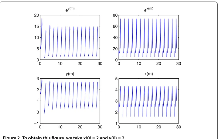
Figure 1 To obtain this figure, we takex(0) = 2 andy(0) = 2.
in []. But although this inequality is satisfied, system () does not have any periodic solu-tion, which means that the predator can go to extinction by Theorem . Therefore, if we are able to extend the conditions that make the predator go to extinction, then we have more information about the systems that have at least one periodic solution.
Example LetT= [k, k+ ],k∈N,kstarting with ,
x(t) =sin(πt) + –.sin(πt) + exp(x)
– ( + cos(πt))exp(y)
(sin(πt) + ) + ( + .cos(πt))exp(x) + exp(y),
y(t) = –.sin(πt) + + (cos(πt) + .)exp(x)
(sin(πt) + ) + ( + .cos(πt))exp(x) + exp(y).
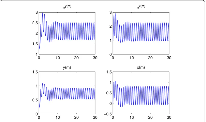
Example LetT= [k, k+ ],k∈N,
x(t) =sin(πt) + –.sin(πt) + exp(x)
– ( + cos(πt))exp(y)
(sin(πt) + ) + ( + .cos(πt))exp(x) + exp(y),
y(t) = –.sin(πt) + + (cos(πt) + .)exp(x)
(sin(πt) + ) + ( + .cos(πt))exp(x) + exp(y).
Figures and satisfy the results obtained in Theorem .
3.2 Continuous case
.. Preliminaries for continuous case
Definition ([]) Solutions of aw-periodic system generate a w-periodic semiflow
Figure 2 To obtain this figure, we takex(0) = 2 andy(0) = 2.
Definition ([]) The periodic semi-flowT(t) is said to be uniformly persistent with respect to (X,∂X) if there exists η> such that for any x∈X, lim inft→∞d(T(t)x,
∂X)≥η.
Definition ([]) LetT :Rn→Rn. The mapT is point dissipative if there exists a bounded set B such that, for each x∈Rn, there is an integer n=n(x,B) such that
Tn(x)∈Bfor eachn≥n
.
Lemma ([]) Let S:X→X be a continuous map with S(X)⊂X.Assume that S is
point dissipative,compact,and uniformly persistent with respect to(X,δX).Then there
exists a global attractor Afor S in Xrelative to strongly bounded sets in X,and S has a
coexistence state x∈A.
Definition ([]) System () is called permanent if there exist positive constantsr,r,
R, andRsuch that solution (x˜(t),y˜(t)) of system () satisfies
r≤ lim
t→∞infx˜(t)≤tlim→∞supx˜(t)≤R,
r≤ lim
t→∞infy˜(t)≤tlim→∞supy˜(t)≤R.
Theorem ([]) Assume that all the coefficient functions in system()are positive.Then system()is permanent and has at least one positive w-periodic solution if
w
w
a(t)dt
–d(t) + f(t)x
∗(t)
α(t) +βx∗(t) > , ()
where x∗(t) = –exp(– w
a(s)ds)
w
b(t–s)exp(–
s
a(t–τ)dτ)ds is the unique global asymptotically stable periodic solution of system()x˜(t) =x˜(t)(a(t) –b(t)˜x(t)).
Corollary ([]) Assume that all the coefficient functions in system()are positive.Then this system is permanent and has at least one w-periodic solution if
fL–dMβMa
b
L
>dMαM, ()
where hMis the maximum of h,and hLis the minimum of h.
Theorem ([]) Assume that all the coefficient functions in system()are positive.Then system()is permanent if and only if inequality()holds.
If we takex˜=exp(x(t)) andy˜=exp(y(t)), then the following system is equivalent to sys-tem():
x(t) =a(t) –b(t)expx(t)– c(t)exp(y(t))
α(t) +β(t)exp(x(t)) +m(t)exp(y(t)),
y(t) = –d(t) + f(t)exp(x(t))
α(t) +β(t)exp(x(t)) +m(t)exp(y(t)).
()
Definition In system (), for all solutions ofx(t) (y(t)), ifexp(x(t)) (exp(y(t))) tends to as t tends to infinity, then we say that the prey (predator) goes to extinction. In other words, in system (), ifx˜(t) (˜y(t)) tends to asttends to infinity, then we say that the prey (predator) goes to extinction.
In [], a sufficient and necessary condition for the permanence of system () is estab-lished by the theorem, which Theorem in this study. Additionally, in the discussion part of that paper, the following corollary is stated.
Corollary ([]) System()goes to extinction if and only if
w
w
a(t)dt
–d(t) + f(t)x
∗(t)
α(t) +βx∗(t) ≤.
.. Application of the main result to the continuous case
Theorem Assume that all the coefficient functions in system()are bounded,positive,
w-periodic,and from C(T,R).Then,there exists at least one w-periodic solution of system
()if and only if inequality()is satisfied.
Proof First, let us assume that inequality () is satisfied. Then system () becomes per-manent by Theorem , and the predator does not go to extinction. Since system () and system () are equivalent, the predator does not go to extinction in system (). Then, by Theorem we obtain that system () has at least onew-periodic solution. Therefore, system () also has at least onew-periodic solution.
For the other part, let us assume that our system () has at least onew-periodic solution. Then system () has at least onew-periodic solution. By Theorem the predator does not go to extinction. By Lemma the prey also does not go to extinction. Thenx˜(t) and ˜
The following lemma is similar to Lemma . in [], but with zero impulses.
Lemma Suppose that inequality()holds.Then,the w-periodic solution of system()
is globally asymptotically stable or globally attractive.
Proof To get the result, we apply Lemma . Let us consider the following ordinary differ-ential equation:
z(t) =Ft,z(t),
z() =φ.
()
HereF∈C([,∞)×R,R),φ∈R,F(t+w,u) =F(t,u). Then, the operator that solves system () can be written as
T(t)z=ze–λt+ t
e–λ(t–s)Fs,T(s)z+λT(s)zds,
whereλis a positive constant. It is obvious thatT() =I. Also, we can verify that
u(s) =
T(s)z, ≤s≤w,
T(s–w)T(w)z, w≤s≤t+w,
is the solution of system () with the initial valueu() =z, wheres∈[,t+w]. By the uniqueness theorem system () has a unique solution; therefore,T(t+w)z=u(t+w) =
T(t)T(w)z.
To apply Lemma , letS=T(w),S=S◦S=T(w)◦T(w) =T(w). Here the considered system () is a periodic system. Therefore, we can apply Theorem and obtain thatT(t) is a compact operator. Additionally, the compactness of the given operator can also be shown by the following alternative way. In [], Theorem ., the considered system is
z(t) =Ft,z(t),
ztk+–z(tk) =Ik
z(tk)
,
z() =φ.
()
HereIk∈C(R,R), and the solution operator of system () is defined as
ˆ
T(t)z=ze–λt+
t
e–λ(t–s)Fs,Tˆ(s)z+λTˆ(s)zds+ <tk<t
e–λ(t–tk)I
k
ˆ
T(tk)z
.
If we takeIkas the zero function, then system () is becomes system (), and the solution
operatorTˆ becomes equal to the solution operatorT. By [] and [],T(t) is a compact operator. ThenSis a compact operator. If we takeX+
i ={zi:zi∈R,zi≥}fori= , and
Xi+={zi:zi∈R,zi> }fori= , , thenX=X+×X+,X=X+×X
+
, andδX=X/X. When
Corollary Assume that all the coefficient functions in system()are bounded,positive,
w-periodic, and from C(T,R).Then,there a globally attractive w-periodic solution for
system()exists if and only if inequality()is satisfied.
Proof Proof is immediate from Lemma and Theorem .
.. Examples for continuous case
Example Consider
x(t) =sin(πt) + –.sin(πt) + .exp(x) – ( + cos(πt))exp(y)
(sin(πt) + .) + ( + .sin(πt))exp(x) +exp(y),
y(t) = –.sin(πt) + .+ (.cos(πt) + .)exp(x)
(sin(πt) + .) + ( + .sin(πt))exp(x) +exp(y).
By some calculations we obtain thatx∗≥exp(– cos(πt)
π )
exp(/π) :=x∗∗. Then we get
–.sin(πt) + .+ (.cos(πt) + .)x
∗(t)
(sin(πt) + .) + ( + .sin(πt))x∗(t) > –.sin(πt) + .+ (.cos(πt) + .)x
∗∗(t)
(sin(πt) + .) + ( + .sin(πt))x∗∗(t)> .
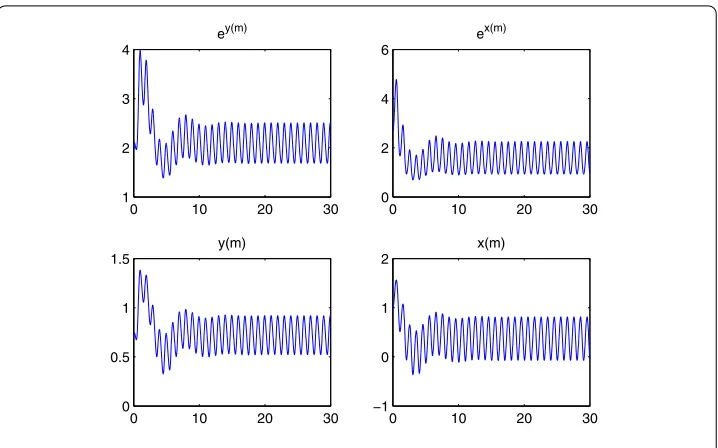
This means that Example satisfies inequality () and has a globally attractive -periodic solution. Figure also supports our findings.
Although we change the initial values of the system in Example , we get the same solu-tion after a while as it is seen in Figure . This shows the global attractivity of the -periodic solution of Example .
Figure 4 To obtain this figure, we takex(0) = 1 andy(0) = 0.7.
For Example , (fL–dMβM)(a
b)L= (. – ()·(.))·() = . anddMαM= ·(.) =
., but . > .. Therefore, this example does not satisfy inequality () in Corollary , but since it satisfies inequality (), we can say that this system has a -periodic globally attractive solution.
Example Consider
x(t) =sin(πt) + –.sin(πt) + exp(x) – ( +cos(πt))exp(y)
(.sin(πt) + ) +exp(x) + exp(y),
y(t) = –.sin(πt) + .+ (cos(πt) + )exp(x) (.sin(πt) + ) +exp(x) + exp(y).
Here the inequality is as follows:
w
–d(t) + f(t) β(t)dt=
–.sin(πt) + .+cos(πt) + dt= . > .
According to the study of [], if the inequality werew–d(t) +βf((tt))dt< , then we could obtain the result that system goes to extinction. However, since we find that this inequality is greater than zero, we cannot make any observation about whether the system goes to extinction or not. For this reason, we use inequality (). After some calculations we obtain thatx∗≤.. Then we get
–.sin(πt) + .+ (cos(πt) + )x
∗(t)
(.sin(πt) + ) +x∗(t) ≤–.sin(πt) + .+ (cos(πt) + ).
(.sin(πt) + ) + .
Figure 5 To obtain this figure we takex(0) = 0.5 andy(0) = 0.3.
Since Example does not satisfy inequality (), the system does not have a periodic solution, the predator of this system goes to extinction, and Figure satisfies this result.
All of the figures in this study are obtained by Matlab program.
4 Discussion
In [], Figure , for the continuous case, there was a discussion about why Figure (a) does not satisfy the conditions of Theorem . in that paper, but the solutions are still periodic. We can answer this question by using our Theorem . When the coefficient functions in Figure (a) are bounded, positive, -periodic, continuous, and the predator does not go to extinction, then we have at least one -periodic solution, which is globally asymptotically stable. Inequality () was first found by Cui and Takeuchi []. However, what they have found was the equivalence between satisfaction of inequality () and the permanence of the predator-prey dynamic systems with Beddington-DeAngelis-type function response. Although they have found that if system () satisfies inequality (), then it has at least onew-periodic solution, they could not say anything about when system () has at least onew-periodic solution, whether it satisfies inequality () or not. In that paper, by using Theorem and Theorem , we can say that for system (), having at least onew-periodic solution of is equivalent to satisfaction of inequality (), which means that a much better development of the inequality for system () to investigate the periodic solution is impos-sible. In addition, by using Corollary we are able to say that satisfaction of inequality () is equivalent to the existence of a globally attractivew-periodic solution.
Hence, for any continuous predator-prey dynamic system with Beddington-DeAngelis-type functional response, there is a globally attractivew-periodic solution if and only if inequality () is satisfied, and the predator of this system goes to extinction if and only if inequality () is not satisfied.
Beddington-DeAngelis functional response for continuous case and for a general time-scale case.
Competing interests
The authors declare that they have no competing interests.
Authors’ contributions
NNP gave the first idea of studying necessary and sufficient conditions of the considered system and also made the literature review. Additionally, NNP desinged the pattern of the study, and all findings were controlled by AFG in each step with BK. NNP participated in the contribution in the mathematical analysis part, and his contributions were controlled by AFG and BK. All of the authors drafted the manuscript together. BK and AFG gave the final approval. All authors read and approved the final manuscript.
Author details
1Department of Mathematics, Ondokuz Mayıs University, Samsun, Turkey.2Department of Mathematics, Faculty of Science, Ankara University, Ankara, 06590, Turkey.3Department of Mathematics and Computer Science, Çankaya University, Ankara, 06810, Turkey.
Acknowledgements
We thank the reviewers and the academic editor of this article for all their contributions in the review process.
Received: 30 July 2015 Accepted: 10 January 2016
References
1. Cui, J, Takeuchi, Y: Permanence, extinction and periodic solution of predator-prey system with Beddington-DeAngelis functional response. J. Math. Anal. Appl.317, 464-474 (2006)
2. Fan, M, Kuang, Y: Dynamics of a nonautonomous predator-prey system with the Beddington-DeAngelis functional response. J. Math. Anal. Appl.295, 15-39 (2004)
3. Wang, W, Shen, J, Nieto, J: Permanence and periodic solution of predator-prey system with Holling type functional response and impulses. Discrete Dyn. Nat. Soc.2007, Article ID 81756 (2007)
4. Bohner, M, Fan, M, Zhang, J: Existence of periodic solutions in predator-prey and competition dynamic systems. Nonlinear Anal., Real World Appl.7, 1193-1204 (2006)
5. Fan, M, Wang, Q: Periodic solutions of a class of nonautonomous discrete time semi-ratio-dependent predator-prey systems. Discrete Contin. Dyn. Syst., Ser. B4(3), 563-574 (2004)
6. Beddington, JR: Mutual interference between parasites or predators and its effect on searching efficiency. J. Anim. Ecol.44, 331-340 (1975)
7. DeAngelis, DL, Goldstein, RA, O’Neill, RV: A model for trophic interaction. Ecology56, 881-892 (1975)
8. Chen, F: Permanence and global stability of nonautonomous Lotka-Volterra system with predator-prey and deviating arguments. Appl. Math. Comput.173, 1082-1100 (2006)
9. Fan, M, Agarwal, S: Periodic solutions for a class of discrete time competition systems. Nonlinear Stud.9(3), 249-261 (2002)
10. Fan, M, Wang, K: Global periodic solutions of a generalizedn-species Gilpin-Ayala competition model. Comput. Math. Appl.40(10-11), 1141-1151 (2000)
11. Fan, M, Wang, K: Periodicity in a delayed ratio-dependent predator-prey system. J. Math. Anal. Appl.262(1), 179-190 (2001)
12. Fang, Q, Li, X, Cao, M: Dynamics of a discrete predator-prey system with Beddington-DeAngelis function response. Appl. Math.3, 389-394 (2012)
13. Huo, HF: Periodic solutions for a semi-ratio-dependent predator-prey system with functional responses. Appl. Math. Lett.18, 313-320 (2005)
14. Li, H, Takeuchi, Y: Dynamics of density dependent predator-prey system with Beddington-DeAngelis functional response. J. Math. Anal. Appl.374, 644-654 (2011)
15. Wang, Q, Fan, M, Wang, K: Dynamics of a class of nonautonomous semi-ratio-dependent predator-prey systems with functional responses. J. Math. Anal. Appl.278(2), 443-471 (2003)
16. Xu, R, Chaplain, MAJ, Davidson, FA: Periodic solutions for a predator-prey model with Holling-type functional response and time delays. Appl. Math. Comput.161(2), 637-654 (2005)
17. Hilger, S: Analysis on measure chains - a unified approach to continuous and discrete calculus. Results Math.18, 18-56 (1990)
18. Fazly, M, Hesaaraki, M: Periodic solutions for predator-prey systems with Beddington-DeAngelis functional response on time scales. Nonlinear Anal., Real World Appl.9, 1224-1235 (2008)
19. Güvenilir, AF, Kaymakçalan, B, Pelen, NN: Impulsive predator-prey dynamic systems with Beddington-DeAngelis type functional response on the unification of discrete and continuous systems. Appl. Math.6, 1649 (2015)
20. Yang, L, Yang, J, Zhog, Q: Periodic solutions for a predator-prey model with Beddington-DeAngelis type functional response on time scales. Gen. Math. Notes3(1), 46-54 (2011)
21. Bohner, M, Peterson, A: Dynamic Equations on Times Scales: An Introduction with Applications. Birkhäuser, Basel (2001)
22. Bourbaki, N: Elements of Mathematics. Algebra: Algebraic Structures. Linear Algebra, 1. Addison-Wesley, Reading (1974) (Chaps. 1, 2)
23. Gaines, RE, Mawhin, JL: Coincidence Degree and Non-Linear Differential Equations. Springer, Berlin (1977) 24. Gong, Y, Xiang, X: A class of optimal control problems of systems governed by the first order linear dynamic
25. Liu, X, Liu, X: Necessary and sufficient conditions for the existence of periodic solutions in a predator-prey model on time scales. Electron. J. Differ. Equ.2012199 (2012)
26. Zhang, J, Wang, J: Periodic solutions for discrete predator-prey systems with the Beddington-DeAngelis functional response. Appl. Math. Lett.19, 1361-1366 (2006)
27. Xu, C, Liao, M: Existence of periodic solutions in a discrete predator-prey system with Beddington-DeAngelis functional responses. Int. J. Math. Math. Sci.2011, Article ID 970763 (2011)
28. Zhao, XQ: Uniform persistence and periodic coexistence states in infinite-dimensional periodic semiflows with applications. Can. Appl. Math. Q.3(4), 473-495 (1995)
29. Hale, JK: Asymptotic Behavior of Dissipative Systems. Math. Surveys and Monographs, vol. 25. Am. Math. Soc., Providence (1988)