Complex dynamic behavior of a discrete time predator prey system of Holling III type

(1)

R E S E A R C H

Open Access

Complex dynamic behavior of a discrete-time

predator-prey system of Holling-III type

Zhimin He

*

_{and Bo Li}

*_{Correspondence:}

[email protected]; [email protected] School of Mathematics and Statistics, Central South University, Changsha, Hunan 410083, People’s Republic of China

Abstract

In this paper, we investigate the dynamics of a discrete-time predator-prey system of Holling-III type in the closed ﬁrst quadrantR2

+. Firstly, the existence and stability of ﬁxed points of the system is discussed. Secondly, it is shown that the system undergoes a ﬂip bifurcation and a Neimark-Sacker bifurcation in the interior ofR2

+by using bifurcation theory. Finally, numerical simulations including bifurcation

diagrams, phase portraits, and maximum Lyapunov exponents are presented not only to explain our results with the theoretical analysis, but also to exhibit the complex dynamical behaviors, such as the period-6, -7, -9, -15, -16, -22, -23, -32, -35 orbits, a cascade of period-doubling bifurcations in period-2, -4, -8, -16 orbits, quasi-periodic orbits, and chaotic sets.

MSC: 37G05; 37G35; 39A28; 39A33

Keywords: discrete dynamical system; predator-prey system; chaos; Lyapunov exponent; stability; period-doubling; ﬂip bifurcation; Neimark-Sacker bifurcation

1 Introduction

The Lotka-Volterra prey-predator model has become one of the fundamental popula-tion models since the theoretical works going back to Lotka () [] and Volterra () [] in the last century. Holling () [] introduced three kinds of functional re-sponses for diﬀerent species to model the phenomena of predation. Qualitative analyses of more realistic prey-predator models can be found in [–]. Recently, there is a grow-ing evidence showgrow-ing that the dynamics of the discrete-time prey-predator models can present a much richer set of patterns than those observed in continuous-time models [–].

In this paper, we consider the predator-prey system of Holling-III type that is given in [] as follows:

⎧ ⎨ ⎩

dx

dt =rx( – x

K) – x

x

x+β,

dx

dt =x(–d+

αx_ x_+β) –γ,

()

wherexandxdenote prey and predator densities, respectively;r,K,α,β,d,γ are

posi-tive constants that stand for prey intrinsic growth rate, carrying capacity, conversion rate, half capturing saturation, the death rate of the predator, the harvesting rate of the predator, respectively. The predator-prey system () assumes that the prey grows logistically with

(2)

intrinsic growth raterand carrying capacityK in the absence of predation. The preda-tor consumes the prey according to the Holling type-III functional responsex

/(x +β)

and contributes to its growth with rateαx

/(x+β). In [], Wanget al.presented a

bi-furcation analysis by choosing the death rate and the harvesting rate of the predator as the bifurcation parameters and proved that system () can undergo the Bogdanov-Takens bifurcation.

Applying the forward Euler scheme to system (), we obtain the discrete-time predator-prey system of Holling-III type as follows:

whereδis the step size. In this paper, we investigate this version as a discrete-time dynam-ical system in the interior of the ﬁrst quadrantR₊by using the normal form theory of the discrete system (see Section  in []; see also [–]), and we prove that this discrete model possesses the ﬂip bifurcation and the Neimark-Sacker bifurcation.

This paper is organized as follows. In Section , we discuss the existence and stabil-ity of ﬁxed points for system () in the closed ﬁrst quadrantR

+. In Section , we show

that there exist some values of the parameters such that () undergoes the ﬂip bifurcation and the Neimark-Sacker bifurcation in the interior of R

+. In Section , we present the

numerical simulations, which not only illustrate our results with the theoretical analysis, but which also exhibit the complex dynamical behaviors such as the period-, -, -, -, -, -, -, -, - orbits, a cascade of period-doubling bifurcations in period-, -, -, - orbits, quasi-periodic orbits, and chaotic sets. The Lyapunov exponents are com-puted numerically to further conﬁrm the dynamical behaviors. A brief discussion is given in Section .

2 The existence and stability of ﬁxed points

It is clear that the ﬁxed points of () satisfy the following equations:

⎧

Next, we consider the existence of the positive ﬁxed points of system (). Suppose that

(3)

Let

Using the Cardano formula (see [, p.]), we have the following results.

Lemma .

Now we study the stability of the ﬁxed points for (). The Jacobian matrixJof system () evaluated at the ﬁxed point (x∗_,x∗_) is given by

and the characteristic equation of the Jacobian matrixJcan be written as

λ–trJλ+detJ= , ()

where

trJ=  +δ(a+b),

detJ=  +δ(a+b) +δ(ab+ab).

(4)

3 Flip bifurcation and Neimark-Sacker bifurcation

In this section, we choose the parameter δas a bifurcation parameter to study the ﬂip bifurcation and the Neimark-Sacker bifurcation of (x∗_,x∗_) by using bifurcation theory in (see Section  in []; see also [–]).

system () into the origin, then system () becomes

(5)

B(x,y) =

We know thatAhas the simple eigenvalueλ(δ) = –, and the corresponding eigenspace

Ec_{is one-dimensional and spanned by an eigenvector}_q_∈_R_{such that}_Aq_{= –}_q_{. Let}_p_∈_R

be the adjoint eigenvector, that is,ATp= –p. By direct calculation we obtain

q∼(– –δb,δa)T,

p∼(– –δb, –δb)T.

In order to normalizepwith respect toq, we denote

p=γ˜(– –δb, –δb)T,

Following the algorithms given in [], the sign of the critical normal form coeﬃcient

c(δ), which determines the direction of the ﬂip bifurcation, is given by the following

for-mula:

From the above analysis and the theorem in [–], we have the following result.

(6)

Figure 1 Bifurcation diagrams and maximum Lyapunov exponent for system (2). (a)Bifurcation diagram of system (2) in (δ,x1) plane ford= 0.05,r= 1.5,K= 1.2,α= 0.8,β= 2.5,γ= 0.1, the initial value is

(0.9, 0.9).(b)Bifurcation diagram of system (2) in (δ,x2) plane.(c)Maximum Lyapunov exponents

corresponding to (a) and (b).

parameterδvaries in a small neighborhood ofδ.Moreover,if c(δ) >  (respectively,c(δ) <

),then the period-orbits that bifurcate from(x∗_,x∗_)are stable(respectively,unstable). In Section  we will give some values of the parameters such thatc(δ)= , thus the ﬂip

bifurcation occurs asδvaries (see Figure ).

We next discuss the existence of a Sacker bifurcation by using the Neimark-Sacker theorem in [–].

The eigenvalues of the characteristic () are

λ,=

trJ±(trJ)_{– }_det_J

 , ()

where

(trJ)– detJ=δ.

The eigenvaluesλ,are complex conjugate for (trJ)– detJ< , which leads to< ,

i.e.,

(7)

Let

δ= –

a+b

ab+ab

, ()

we havedetJ(δ) = .

Forδ=δ, the eigenvalues of the matrix associated with the linearization of the map ()

at (x˜,x˜) = (, ) are conjugate with modulus , and they are written as

λ,λ¯=trJ(δ)

 ±

i



detJ(δ) –

trJ(δ)



=  +δ

(a+b)±

iδ



ab– (a–b) ()

and|λ(δ)|= , d|λ_d(_δδ)||δ=δ= –

a+b

 = .

In addition, iftrJ(δ)= , –, which leads to

δ(a+b)= –, –, ()

then we haveλk(δ)=  fork∈ {, , , }.

Letq∈Cbe an eigenvector ofA(δ) corresponding to the eigenvalueλ(δ) such that

A(δ)q=λ(δ)q, A(δ)q¯=λ(δ)q¯.

Also letp∈C be an eigenvector of the transposed matrixAT(δ) corresponding to its

eigenvalue, that is,λ(δ),

AT(δ)p=λ(δ)p, AT(δ)p¯=λ(δ)p¯.

By direct calculation we obtain

q∼( +δb–λ, –δa)T,

p∼( +δb–λ¯,δb)T.

In order to normalizepwith respect toq, we denote

p=γ( +δb–λ¯,δb)T,

where

γ = 

( +δb–λ¯)–δab

.

It is easy to see that p,q= , where ·,·means the standard scalar product inC_: _p_,_q₌

¯

pq+p¯q.

Any vectorx∈Rcan be represented forδnearδas

(8)

for some complexz. Obviously,z= p,x. Thus, system () can be transformed forδnear

¯

δ∗into the following form:

z→λ(δ)z+g(z,z¯,δ),

whereλ(δ) can be written asλ(δ) = ( +ϕ(δ))eiθ(δ)₍_ϕ₍_δ_{) is a smooth function with}_ϕ₍_δ ) = )

andg is a complex-valued smooth function ofz,z¯, andδ, whose Taylor expression with respect to (z,z¯) contains quadratic and higher-order terms:

g(z,z¯,δ) =

For the above argument and the theorem in [–], we have the following result.

Theorem . Suppose that(x∗_,x∗_)is the positive ﬁxed point.If a(δ) <  (respectively, > )

the Neimark-Sacker bifurcation of system()atδ=δis supercritical(respectively,

subcrit-ical)and there exists a unique closed invariant curve bifurcation from(x∗,x∗)forδ=δ,

which is asymptotically stable(respectively,unstable).

In Section  we will choose some values of the parameters so as to show the process of a Neimark-Sacker bifurcation for system () in Figure  by numerical simulation.

4 Numerical simulations

In this section, we present the bifurcation diagrams, phase portraits, and maximum Lyapunov exponents for system () to explain the above theoretical analysis and show the new interesting complex dynamical behaviors by using numerical simulations. The bifurcation parameters are considered in the following three cases:

(9)

Figure 2 Bifurcation diagrams and maximum Lyapunov exponent for system (2). (a)Bifurcation diagram of system (2) in (δ,x1) plane ford= 2,r= 2,K=85,α= 3,β=

1 3,γ=

1

4, the initial value is (0.89, 0.87).

(b)Bifurcation diagram of system (2) in (δ,x2) plane.(c)Maximum Lyapunov exponents corresponding to (a)

and (b).

of period-doubling bifurcations in period-, -, -, - orbits. The maximum Lyapunov exponents corresponding to Figure (a) and (b) are calculated and plotted in Figure (c), conﬁrming the existence of the chaotic regions and period orbits in the parametric space. Case (). The bifurcation diagrams of system () in the (δ,x) and (δ,x) plane ford= ,

r= ,K=_,α= ,β=_,γ=_ are given in Figure (a) and (b), respectively. After calcu-lation for the positive ﬁxed point of system (), the Neimark-Sacker bifurcation emerges from the ﬁxed point (, ) atδ= , and its eigenvalues areλ±= .±.i. Forδ= ,

we have|λ±|= ,l=d_d|λ_δ||δ=δ= . > ,g= –. – .i,g= . – .i, g= . + .i,g= –. + .i,a(δ) = –.. It shows the correctness

of Theorem ..

(10)

Figure 3 Bifurcation diagrams and maximum Lyapunov exponent for system (2). (a)Local ampliﬁcation corresponding to Figure 1(a) forδ∈[1.488, 1.588].(b)Local ampliﬁcation corresponding to Figure 1(a) for δ∈[1.608, 1.616].(c),(d)Maximum Lyapunov exponents corresponding to (a) and (b), respectively.

(11)

Figure 5 Bifurcation diagrams and maximum Lyapunov exponent for system (2). (a)Bifurcation diagram of system (2) in the (r,x1) plane ford= 2,δ= 1,K=85,α= 3,β=

1 3,γ=

1

4, the initial value is

(0.89, 0.87).(b)Bifurcation diagram of system (2) in the (r,x2) plane.(c)Maximum Lyapunov exponents

corresponding to (a) and (b).

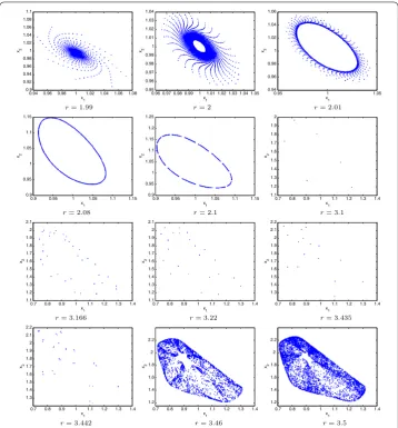
The phase portraits which are associated with Figure (a) and (b) are revealed in Fig-ure , which clearly depicts the process of how a smooth invariant circle bifurcates from the stable ﬁxed point (, ). Whenδexceeds  there appears a circle curve enclosing the ﬁxed point (, ), and its radius becomes larger with respect to the growth ofδ. Whenδ increases at certain values, for example, atδ= ., the circle disappears and a period- orbit appears. From Figure , we observe that there are period-, -, -, - orbits, quasi-periodic orbits, and attracting chaotic sets.

Case (). The bifurcation diagrams of system () in the (r,x) and (r,x) plane ford= ,

δ= ,K=

,α= ,β=  ,γ =



are given in Figure (a) and (b), respectively. After

calcu-lation for the positive fixed point of system (), the Neimark-Sacker bifurcation emerges from the fixed point (, ) atr= . From Figure (a) and (b), we observe that the fixed point of map () is stable forr< , loses its stability atr= , and an invariant circle appears when the parameterrexceeds .

The maximum Lyapunov exponents corresponding to Figure (a) and (b) are calculated and plotted in Figure (c). Forr∈(., .), some Lyapunov exponents are bigger than , some are smaller than , which implies that there exist stable ﬁxed points or stable period windows in the chaotic region.

(12)

Figure 6 Phase portraits for various values ofrcorresponding to Figure 5(a) and (b).

5 Conclusion

In this paper, we investigate the complex behaviors of the discrete-time predator-prey sys-tem of Holling-III type obtained by the Euler method in the closed ﬁrst quadrantR

+, and

we show that system () can undergo a ﬂip bifurcation and a Neimark-Sacker bifurcation in the interior ofR

+. Moreover, system () displays very interesting dynamical behaviors,

including period-, -, -, -, -, -, -, -, - orbits, a cascade of period-doubling bifurcations in period-, -, -, - orbits, an invariant cycle, quasi-periodic orbits, and chaotic sets. These results reveal far richer dynamics of the discrete-time models com-pared to the continuous-time models.

Competing interests

The authors declare that they have no competing interests.

Authors’ contributions

All authors contributed equally to the writing of this paper. All authors read and approved the ﬁnal manuscript.

(13)

References

1. Lotka, AJ: Elements of Mathematical Biology. Dover, New York (1956)

2. Volterra, V: Opere Matematiche: Memorie e Note, vol. V. Acc. Naz. dei Lincei, Roma (1962)

3. Holling, CS: The functional response of predator to prey density and its role in mimicry and population regulation. Mem. Entomol. Soc. Can.45, 1-60 (1965)

4. Collings, JB: Bifurcation and stability analysis of a temperature-dependent mite predator-prey interaction model incorporating a prey refuge. Bull. Math. Biol.57, 63-76 (1995)

5. Collings, JB, Wollking, DJ: A global analysis of a temperature-dependent model system for a mite predator-prey interaction. SIAM J. Appl. Math.50, 1348-1372 (1990)

6. Freedman, HI, Mathsen, RM: Persistence in predator-prey systems with ratio-dependent predator inﬂuence. Bull. Math. Biol.55, 817-827 (1993)

7. Hastings, A: Multiple limit cycles in predator-prey models. J. Math. Biol.11, 51-63 (1981)

8. Lindström, T: Qualitative analysis of a predator-prey systems with limit cycles. J. Math. Biol.31, 541-561 (1993) 9. Murray, JD: Mathematical Biology: I. An Introduction, 3rd edn. Springer, New York (2002)

10. Ruan, S, Xiao, D: Global analysis in a predator-prey system with nonmonotonic functional response. SIAM J. Appl. Math.61, 1445-1472 (2001)

11. Sáez, E, González-Olivares, E: Dynamics of a predator-prey model. SIAM J. Appl. Math.59, 1867-1878 (1999) 12. Agiza, HN, Elabbasy, EM, El-Metwally, H, Elsadany, AA: Chaotic dynamics of a discrete prey-predator model with

Holling type II. Nonlinear Anal., Real World Appl.10, 116-129 (2009)

13. Beddington, JR, Free, CA, Lawton, JH: Dynamic complexity in predator-prey models framed in diﬀerence equations. Nature255, 58-60 (1975)

14. Danca, M, Codreanu, S, Bako, B: Detailed analysis of a nonlinear prey-predator model. J. Biol. Phys.23, 11-20 (1997) 15. Hadeler, KP, Gerstmann, I: The discrete Rosenzweig model. Math. Biosci.98, 49-72 (1990)

16. He, ZM, Lai, X: Bifurcations and chaotic behavior of a discrete-time predator-prey system. Nonlinear Anal., Real World Appl.12, 403-417 (2011)

17. Jing, ZJ, Yang, J: Bifurcation and chaos in discrete-time predator-prey system. Chaos Solitons Fractals27, 259-277 (2006)

18. Jing, ZJ, Jia, ZY, Wang, RQ: Chaos behavior in the discrete BVP oscillator. Int. J. Bifurc. Chaos12(3), 619-627 (2002) 19. Johnson, P, Burke, M: An investigation of the global properties of a two-dimensional competing species model.

Discrete Contin. Dyn. Syst., Ser. B10, 109-128 (2008)

20. Liu, X, Xiao, D: Complex dynamics behaviors of a discrete-time predator-prey system. Chaos Solitons Fractals32, 80-94 (2007)

21. Lopez-Ruiz, R, Fournier-Prunaret, R: Indirect Allee eﬀect, bistability and chaotic oscillations in a predator-prey discrete model of logistic type. Chaos Solitons Fractals24, 85-101 (2005)

22. Summers, D, Cranford, JG, Healey, BP: Chaos in periodically forced discrete-time ecosystem models. Chaos Solitons Fractals11, 2331-2342 (2000)

23. Xiao, YN, Cheng, DZ, Tang, SY: Dynamic complexities in predator-prey ecosystem models with age-structure for predator. Chaos Solitons Fractals14, 1403-1411 (2002)

24. Wang, LL, Fan, YH, Li, WT: Multiple bifurcations in a predator-prey system with monotonic functional response. Appl. Math. Comput.172, 1103-1120 (2006)

25. Kuznetsov, YK: Elements of Applied Bifurcation Theory, 3rd edn. Springer, New York (1998)

26. Guckenheimer, J, Holmes, P: Nonlinear Oscillations, Dynamical Systems, and Bifurcations of Vector Fields. Springer, New York (1983)

27. Robinson, C: Dynamical Systems, Stability, Symbolic Dynamics and Chaos, 2nd edn. CRC Press, Boca Raton (1999) 28. Wiggins, S: Introduction to Applied Nonlinear Dynamical Systems and Chaos, 2nd edn. Springer, New York (2003) 29. Polyanin, AD, Chernoutsan, AI: A Concise Handbook of Mathematics, Physics, and Engineering Science. CRC Press,

New York (2011)

30. Elaydi, SN: An Introduction to Diﬀerence Equations, 3rd edn. Springer, New York (2005)

31. Alligood, KT, Sauer, TD, Yorke, JA: Chaos - An Introduction to Dynamical Systems. Springer, New York (1996) 32. Ott, E: Chaos in Dynamical Systems, 2nd edn. Cambridge University Press, Cambridge (2002)

10.1186/1687-1847-2014-180