Efficient Algorithms for Computing Differential Properties of Addition

(1)

Efficient Algorithms for Computing Differential

Properties of Addition

Helger Lipmaa and Shiho Moriai

Helsinki University of Technology, Department of Computer Science and Engineering P.O.Box 5400, FI-02015 HUT, Espoo, Finland

[email protected] NTT Laboratories

1-1 Hikari-no-oka, Yokosuka, 239-0847 Japan [email protected]

Abstract. In this paper we systematically study the differential properties of ad-dition modulo

. We derive -time algorithms for most of the properties, including differential probability of addition. We also present log-time algorithms for finding good differentials. Despite the apparent simplicity of modular addi-tion, the best known algorithms require naive exhaustive computation. Our re-sults represent a significant improvement over them. In the most extreme case, we present a complexity reduction from

to .

Keywords: modular addition, differential cryptanalysis, differential probability,

impos-sible differentials, maximum differential probability.

1 Introduction

One of the most successful and influential attacks against block ciphers is Differential Cryptanalysis (DC), introduced by Biham and Shamir in 1991 [BS91a]. For many of the block ciphers proposed since then, provable security against DC (defined by Lai, Massey and Murphy [LMM91] and first implemented by Nyberg and Knudsen [NK95]) has been one of the primary criteria used to confirm their potential quality.

Unfortunately, few approaches to proving security have been really successful. The original approach of [NK95] has been used in designing MISTY and its variant KA-SUMI (the new 3GPP block cipher standard). Another influential approach has been the “wide trail” strategy proposed by Daemen [Dae95], applied for example in the pro-posed AES, Rijndael. The main reason for the small number of successful strategies is the complex structure of modern ciphers, which makes exact evaluation of their differ-ential properties infeasible. This has, unfortunately, led to a situation where the security against DC is often evaluated by heuristic methods.

We approach the above problem by using the bottom-up methodology. That is, we evaluate many sophisticated differential properties of one of the most-used “non-trivial”

block cipher cornerstones, addition modulo for! . We hope that this will help

(2)

results will facilitate cryptanalysis of such stream ciphers and hash functions that use addition and XOR at the same time.

Importance of Differential Properties of Addition. Originally, DC was considered

with respect to XOR, and was generalized to DC with respect to an arbitrary group operation in [LMM91]. In 1992, Berson [Ber92] observed that for many primitive op-erations, it is significantly more difficult to apply DC with respect to XOR than with respect to addition modulo"

. Most interestingly, he classified DC of addition modulo

itself, with sufficiently big, with respect to XOR to be hard to analyze, given the

(then) current state of theory.

Until now it has seemed that the problem of evaluating the differential properties of addition with respect to XOR is hard. Hereafter, we omit the “with respect to XOR” and

take the addition to be always modulo . The fastest known algorithms for computing

the differential probability of addition#%$'&)(+*',.-0/132547698%:<;>=?A@B(DCFEHGI4JK(.(DCLJH*4ME

(DGJN-4O4P8Q2R is exponential in . The complexity of the algorithms for the maximum

differential probability #S$ &TU+V

(+*',.-4W68YX[Z\A]'#S$

&

(^*_,O-0/13254 , the double-maximum

differential probability#%$ &` TU+V

(+*4a698YXbZc\ed

=

]_#S$

&

(^*_,O-0/13254 , and many other

differ-ential properties of addition are also expondiffer-ential in .

With small (e.g.,H8gf or even withH8h i ), exponential-in- computation is

feasible, as demonstrated in the cryptanalysis of FEAL by Aoki, Kobayashi and Moriai

in [AKM98]. However, this is not the case whenHkjl as used in the recent 128-bit

block ciphers such as MARS, RC6 and Twofish. In practice, ifmnjl , both cipher

designers and cryptanalysts have mostly made use of only a few differential properties

of addition. (For example, letting Co be the least significant bit of C , they often use

the property that *po<Jq-ro<JQ2sot83u .) It means that block ciphers that employ both

XOR and addition modulo are hard to evaluate the security against DC due to the

lack of theory. This has led to the general concern that mixed use of XOR and modular addition might add more confusion (in Shannon’s sense) to a cipher but “none has yet demonstrated to have a clear understanding of how to produce any proof nor convincing arguments of the advantage of such an approach” [Knu99]. One could say that they also add more confusion to the cipher in the layman’s sense.

There has been significant ongoing work on evaluating the security of such “confus-ing” block ciphers against differential attacks. Some of these papers have also somewhat focused on the specific problem of evaluating the differential properties of addition. The

full version of [BS91b] treated some differential probabilities of addition modulo

and included a few formulas useful to compute#%$ & , but did not include any concrete

algorithms nor estimations of their complexities. The same is true for many later papers that analyzed ciphers like RC5, SAFER, and IDEA. Miyano [Miy98] studied the sim-pler case with one addend fixed and derived a linear-time algorithm for computing the corresponding differential probability.

Our Results. We develop a framework that allows the extremely efficient evaluation

of many interesting differential properties of modular addition. In particular, most of

the algorithms described herein run in time, sublinear in . Since this would be

(3)

Access Machine) model, which executes basic -bit operations like Boolean operations

and addition modulo> in unit time, as almost all contemporary microprocessors do.

The choice of this model is clearly motivated by the popularity of such micropro-cessors. Still, for several problems (although sometimes implicitly) we also describe linear-time algorithms that might run faster in hardware. (Moreover, the linear-time algorithms are usually easier to understand and hence serve an educational purpose.) Nevertheless, the RAM model was chosen to be “minimal”, such that the described algorithms would be directly usable on as many platforms as possible. On the other hand, we immediately demonstrate the power of this model by describing some useful log-time algorithms (namely, for the Hamming weight, all-one parity and common al-ternation parity). They become very useful later when we investigate other differential properties. One of them (for the common alternation parity) might be interesting by itself; we have not met this algorithm in the literature.

After describing the model and the necessary tools, we show that#S$_& can be

com-puted in timev[(DwBx>y_p4 in the worst-case. The corresponding algorithm has two

princi-pal steps. The first step checks in constant-time whether the differentialz<8{(+*',.-0/13254

is impossible (i.e., whether#S$ & (^z4|8Qu ). The second step, executed only ifz is

possi-ble, computes the Hamming weight of an -bit string in timev[(DwBx>y_p4. As a corollary,

we prove an open conjecture from [AKM98].

The structure of the described algorithm raises an immediate question of what is

the density of the possible differentials. We show that the event #S$_&}(^z4q~8u

oc-curs with the negligible probability s

e (This proves an open conjecture stated

in [AKM98]). That is, the density of possible differentials is negligible, so#%$

& can be

computed in time v[( 4 in the average-case. These results can be further used for

im-possible differential cryptanalysis, since the best previously known general algorithm to find non-trivial impossible differentials was by exhaustive search. Moreover, the high density of impossible differentials makes differential cryptanalysis more efficient; most of the wrong pairs can be filtered out [BS91a,O’C95].

Furthermore, we compute the explicit probabilities:<l@#%$ & (+z4|8R for any7,|u

. This helps us to compute the distribution of the random variable 6zH/1

#S$ & (^z4, and to create formulas for the expected value and variance of the random

variable . Based on this knowledge, one can easily compute the probabilities that

:b@R for any.

For the practical success of differential attacks it is not always sufficient to pick a random differential hoping it will be “good” with reasonable probability. It would be nice to find good differentials efficiently in a deterministic way. Both cipher designers and cryptanalysts are especially interested in finding the “optimal” differentials that re-sult in the maximum differential probabilities and therefore in the best possible attacks. For this purpose we describe a log-time algorithm for computing#S$_&TU+V (^*_,O-4 and a2

that achieves this probability. Both the structure of the algorithm (which makes use of the all-one parity) and its proof of correctness are nontrivial. We also describe a

log-time algorithm that finds a pair(D-|,O24 that maximizes the double-maximum differential

probability#%$'&` TU+V (^*M4. We show that for many nonzero* -s,#S$_&` TU+V (+*4 is very close

(4)

B

Previous result

l¡

H ¢£e¡

s¡ Our result (worst-case), ¥¤a (average) ¦M

Table 1. Summary of the efficiency of our main algorithms

Road map. We give some preliminaries in Sect. 2. Section 3 describes a unit-cost

RAM model, and introduces the reader to several efficient algorithms that are crucial for the later sections. In Sect. 4 we describe a log-time algorithm for#S$_& . Section 5

gives formulas for the density of impossible differentials and other statistical properties of #S$ & . Algorithms for maximum differential probability and related problems are

described in Sect. 6.

2 Preliminaries

Let §¨8ª©uI, « be the binary alphabet. For any -bit stringC¬§ , let C®¯¬§

be the -th coordinate ofC (i.e.,C8±°

e ®³² o

C ®

®

). We always assume thatC ® 8nu if

)~¬´@ur,O¶µ R. (That is,C¶8 °¸·

·

C ®

®

.)

Let J , ¹ , º and » denote -bit bitwise “XOR”, “OR”, “AND” and “negation”,

respectively. LetC¼½ (resp.C¾½) denote the right (resp. the left) shift by positions

(i.e.,C}¼m768À¿DCÂÁ> ®Ã

andC)¾m7698%

®

C3X[xAÄ¯ ). Addition is always performed modulo

, if not stated otherwise. For anyC ,G andÅ we defineÆÇ(DC,OGÂ,.Åe4W68(+»CJGI4Wº(»CJÅe4

(i.e.,ÆÇ(DC,OGÂ,.Åe4®M8{ KÈÉ C®Ê8QG>®8qÅ®) andËcÌeÍ(DC,OGÂ,.Åe4W68CJG<JÅ . For any , let ÎSÏÐaÑ

(^p4W68 µH . For example,(.(+»Mul4s¾ 4o 8Qu .

Addition moduloÒIÓ . The carry,Ô

Ï

ÍÍBÕA(^Cp,.GA4a698%Ö%¬Y§ ,Cp,OGÀ¬×§ , of additionC'EbG is

defined recursively as follows. First,Öao>68%u . Second,Ö ®

&

68(DC ®ºG ®4.J(^C ®ºMÖ ®4.J(^G ® ºMÖ ®4,

for everyP¸u . Equivalently,Öa®

&

8½ KÈ[É C®ENGl®E Öa®'Q . (That is, the carry bit

Öa®

&

is a function of the sumC®lEG>®>EYÖa®.) The following is a basic property of addition

modulo .

Property 1. If(DC,OGI4P¬§LØ§ , thenCENG[8¸CJÙGJÔ

Ï

Í+ÍBÕI(DCp,.GI4 .

Differential Probability of Addition. We define the differential of addition modulo

as a triplet of two input and one output differences, denoted as(+*',.-H/1ª254, where

*',.-|,2Y¬Y§ . The differential probability of addition is defined as follows:

#S$ & (^z4'8¸#S$ & (^*_,O-0/13254W68%: ;>=? @B(DCbEÙGI45JQ(O(^C[J*4pEQ(DG<JÙ-4O4'82RbÚ

That is,#S$ & (^z4W68 Û7©Cp,.GL6r(^CEÙGI45J¸(O(DCbJÙ*M4pEQ(DG JN-4.4'8H2«cÁ>

. We say thatz is impossible if#%$ & (+z4'8Qu . Otherwise we say thatz is possible. It follows directly from

Property 1 that one can rewrite the definition of#S$ & as follows:

Lemma 1. #%$ & (^*_,O-0/1Ü24|8¸:<;=?A@Ô

Ï

Í+ÍBÕr(DC,OGI4>JÀÔ

Ï

(5)

Probability Theory. Let be a discrete random variable. Except for a few

explic-itly mentioned cases, we always deal with uniformly distributed variables. We note

that in the binomial distribution, :b@Ý8ßÞsR¯8áàâA(O bµà4OeÂâ

â

869ãM(+ÞÂä.Ê,^à4, for

some fixed umåàæ and any Þ!¬èç£ç

&

. From the basic axioms of probabil-ity, °

â

² o

ãM(ÞÂäOÊ,+à4L8 . Moreover, the expectation é@R<8 °

â

² o

Þ

:b@ê8ÜÞsR

of a binomially distributed random variable is equal to Aà , while the variance

ë ìIí

@×R8Qé@

Rµ´é@×R

is equal toAà( }µ¶à4.

3 RAM Model and Some Useful Algorithms

In the -bit unit-cost RAM model, some subset of fixed -bit operations can be

exe-cuted in constant time. In the current paper, we specify this subset to be a small set of

-bit instructions, all of which are readily available in the vast majority of contemporary

microprocessors: Boolean operations, addition, and the constant shifts. We additionally allow unit-cost equality tests and (conditional) jumps. On the other hand, our model does not include table look-ups or (say) multiplications. Such a restriction guarantees that algorithms efficient in this model are also efficient on a very broad class of plat-forms, including FPGA and other hardware. This is further emphasized by the fact that our algorithms need only a few bytes of extra memory and thus a very small circuit size in hardware implementations.

Many algorithms that we derive in the current paper make heavy use of the three non-trivial functions described below. The power of our minimal computational model is stressed by the fact that all three functions can be computed in timev[(^w³xly'p4.

Hamming Weight. The first function is the Hamming weight function (also known as

the population count or, sometimes, as sideways addition)î}ï : ForCq8 °

e ®B² o

C®¥

®

,

î ï (^C4À8 ° e ®³² o

C ®, i.e.,î ï counts the “one” bits in an -bit string. In the unit-cost

RAM model,î ï (DCÂ4 can be computed in v[(DwBx>y'p4 steps. Many textbooks contain (a

variation of) the next algorithm that we list here only for the sake of completeness.

INPUT:C

OUTPUT:î ï (DC4

1. C¶ðÜCFµ(O(^Cñ¼ 45º¯òlóAôeôeôeôeôsôeôeôsõ4;

2. C¶ðö(^Cº¯ò>óI÷e÷e÷e÷s÷e÷e÷e÷sõ4E¸(.(DCñ¼m>4pº¶òlóI÷s÷e÷e÷e÷e÷s÷e÷sõ4;

3. C¶ðö(^CE¸(^Cñ¼Køe4O4º¶òlóIòlùIò>ùIòlùIòlùeõ ;

4. C¶ðÜCEQ(DCP¼kfl4;

5. C¶ðö(^CE¸(^Cñ¼ il4.45º¯ò>óIòeòeòeòsòeòe÷lùAõ ;

6. ReturnC ;

Additional time-space trade-offs are possible in calculating the Hamming weight. If

×8qÖWú , then one can precompute>û values ofî ï (D4 ,u[H'ü>û , and then findî ï (DC4

by doingú8KÁcÖ table look-ups. This method is faster than the method described in

the previous paragraph ifúª{wBx>y

, which is the case ifH8gjs andúö¬©fr, iA« .

(6)

%þNÿWÿÿÿÿÿÿÿÿÿÿÿÿÿWÿWÿWÿÿÿ7ÿWÿcÿ

ý

þNÿÿÿÿWÿÿÿÿÿWÿÿÿWÿÿÿÿÿÿWÿWÿWÿ7ÿWÿcÿ

ý

þNÿÿÿÿWÿÿÿÿÿÿWÿÿÿWÿÿÿÿÿWÿWÿWÿ7ÿWÿcÿ

ý

þNÿÿÿÿÿÿÿÿÿÿÿÿÿÿÿÿWÿÿÿÿÿ7ÿÿWÿÿWÿaÿ

ý

þNÿÿÿÿÿÿÿÿÿÿÿÿÿÿÿWÿÿÿÿÿWÿÿWÿÿ7ÿWÿcÿ

Fig. 1. A pair ý

with corresponding values

ý

,

ý

,

ý and

ý . Here, for example,

ý

þ

¤ since¤ þý

þý

and0

þ

¤ is odd. On the other hand,

ý

þ

¤ since

ý

þ

þ´ý

¢

þ

¢

þ´ý

þ

þÙý

þ

þ´ý! |þ , and"

$# is even. Since%'&

þ

#

, we could have taken also

ý( &

þ

¤

Interestingly, many ancient and modern power architectures have a special

machine-level “cryptanalyst’s” instruction forî ï (mostly known as the population count

instruc-tion): SADDon the Mark I (sic),CX X) on the CDC Cyber series, A PS) on the

Cray X-MP,VPCNTon the NEC SX-4,CTPOPon the Alpha 21264,POPCon the

Ul-tra SPARC,POPCNTon the Intel IA64, etc. In principle, we could incorporate in our

model a unit-time population count instruction, then several later presented algorithms would run in constant time. However, since there is no population count instruction on most of the other architectures (especially on the widespread Intel IA32 platform), we have decided not include it in the set of primitive operations. Moreover, the complexity of population count does not significantly influence the (average-case) complexity of the derived algorithms.

All-one and Common Alternation Parity. The second and third functions, important

for several derived algorithms (more precisely, they are used in Algorithm 4 and

Al-gorithm 5), are the all-one and common alternation parity of -bit strings, defined as

follows. (Note that while the Hamming weight has very many useful applications in cryptography, the functions defined in this section have never been, as far as we know, used before for any cryptographic or other purpose.)

The all-one parity of an -bit numberC is another -bit number GÙ8

Ï

Ì+*e(DCÂ4 s.t.

G

®

8 iff the longest sequence of consecutive one-bitsC

®

C

®

&

ÚÚÚOC

®

&,

8 l |ÚÚÚW has

odd length.

The common alternation parity of two -bit numbersC andG is a function-[(^Cp,.GA4

with the next properties: (1)-[(DC,OGI4® 8{ , if. ® is even and non-zero, (2)-[(^Cp,OGI4® 8Qu ,

if. ® is odd, (3) unspecified (eitheru or ) if. ® 8¸u , where. ® is the length of the longest

common alternating bit chainC ® 8kG ® ~8{C ®

&

8{G ®

&

~

8kC ®

&

8kG ®

&

ÚÚÚÊ~8kC ® &0/1

8

G ® &0/1

, whereE2. ® q×µ . (In both cases, counting starts with one. E.g., ifC ® 8kG ®

butC®

&

~8¸G>®

&

then.®p8{ and-[(^Cp,OGI4O®8¸u .) W.l.o.g., we will define

-[(^Cp,.GA4a698

Ï

Ì3*e(»P(DCJNGI45ºt(+»P(^CJÙGI4s¼ 4ºt(^CJ¸(^Cñ¼ 4O4.4tÚ

For both the all-one and common alternation parity we will also need their

“du-als” (denoted as Ï

(7)

Algorithm 1 Log-time algorithm forÏ Ì3*s(DCÂ4 INPUT:ý87$9

, is a power of

OUTPUT:

ý

1. ý;: ¤=<

þ´ý>

ý@? ¤W; 2. ForA;B

to

¤ do ý:

AC<!B ý;:

A

¤D<

>

ý;:

A

¤D<

?

ECF

; 3. +:

¤D<!B

ý>HGÂý;: ¤D<; 4. ForA;B

to

do +:

AC<!B +:

A

¤D<IF£ 3:

A

¤=<

?

EJF

>ý;:

A

¤D<B; 5. Return+:

!<;

Ï

Ì+*4l(DC,OGI4'8

Ï

Ì3*e(^CK,OG!K4, whereCK® 68¸C e

® and G!K® 68G

e

®. (See Fig. 1.) Note that for

every(DC,OGI4 and,-[(DC,OGI4

®

8K SÉL-[(^Cp,OGI4

®

&

8M-[(^Cp,OGI4

®

8u .

Clearly, Algorithm 1 finds the all-one parity ofC in timev[(^w³xly'p4 . (It is sufficient

to note that C@R

,

8 if and only if the number

,

of ones in the sequence (DC

,

8

>,OC ,.&

8 l,ÚÚÚa,.C ,.&

5N

8 l,OC ,.&

5Na

8±ul4 is at least

®

andG@R

,

8 iff

,

is

an odd number not bigger than

, .) Therefore also

-[(^Cp,OGI4 can be computed in time

v[(DwBx>y'p4.

4 Log-time Algorithm for Differential Probability of Addition

In this section we say that differentialz×83(+*',.- /1 254 is “good” ifÆÇ(^*¾á l,O-¶¾

>,2¾ 4}º (ËÌeÍ(^*_,O-',254J (+* ¾ 4O4N8ßu . Alternatively, z is not “good” iff for

some Q¬ö@uI,Oµ! R, * ®

8¨- ®

8 2 ®

~8 * ® J½- ® Jm2 ®. (Remember that

*

8Q-

8¸2

8qu .) The next algorithm has a simple linear-time version, suitable

for “manual cryptanalysis”: (1) Check, whetherz is “good”, using the second definition

of “goodness”; (2) Ifz is “good”, count the number of positions)~8¸µ , s.t. the triple

(^* ® ,.- ® ,2 ®4 contains both zeros and ones.

Theorem 1. Let z8(+*',.-h/1254 be an arbitrary differential. Algorithm 2 returns

#S$ & (^z4 in timev[(DwBx>y'p4. More precisely, it works in timev[(O 4IEPO, whereO is the time it takes to computeî}ï .

Algorithm 2 Log-time algorithm for#%$ & INPUT:Q

þ

CR SUTVXW

OUTPUT:P CQ

1. IfYDZsCR\[ ¤ (S

[K¤ W

[ ¤W

>

^] `_

CR SaW

3bN

S

[ ¤W£

þ

#

then return# ; 2. Return FcdfehgiCjelknmompqsr

cstvu e F

qsq ;

Rest of this subsection consists of a step-by-step proof of this result, where we use the Lemma 1, i.e., that#S$ & (^z4|8Q:<;=?e@Ô

Ï

Í+ÍBÕr(DC,OGI4 J<Ô

Ï

(8)

We first state and prove two auxiliary lemmas. After that we show how Theorem 1 follows from them, and present two corollaries.

Lemma 2. Letw(^C4 be a mapping, such thatw(^us4|8u ,w( 4Ê8xwS(+>4Ê8 and

w(+jl4Ê8 . Let*_,O-Ù¬Y§ . Then:<;>=?A@Ô

Ï Í+ÍBÕr(DC,OGI4® & J Ô Ï ÍÍ³ÕI(DCbJN*_,OGJN-4 ® &

8{ y* ® EÙ- ® E

z

Ö ® 8{)>R8xw(^)s4.

Proof. We denote Öb8!Ô

Ï

ÍÍ³Õr(^Cp,.GA4 andÖ|b8 Ô

Ï

Í+ÍBÕr(DCÀJ¸*',.GJH-4, whereC andG are

understood from the context. Let alsoz

Ö)8QÖÂJÖ| . By the definition of carry,

z Öa® & 8 (DC®º)G>®¥4JY(DC®ºÖa®¥4JY(DG>®aºSÖa®¥4J(.(DC_JL*4O®º (^GMJF-4®¥4JY(O(DC_JL*M4®ºSÖ| ® 4J(.(DGÊJb-4O®ºSÖ| ® 4.

This formula for

z

Öa®

&

is symmetric in the three pairs (DC® ,.*®+4 ,(^G>®O,.-®4 and(+Öa®O,

z

Öa®4.

Hence, the function}M(^*®,.-®.,

z Öa®4W68%: ; 1 =? 1 = û 1 @ z Öa® &

8½ R is symmetric, and therefore

} is a function of*®lE-®>E

z

Öa®,}M(^)e4|8¸: ;

1 =? 1 = û 1 @ z Öa® &

8{ y*®>E×-®>E

z

Öa®8~)>R. One

can now prove that:<;

1 =? 1 @ z Ö ® &

8m y* ® EÙ- ® E

z

Ö ® 8~)>Rp8w(v)e4 for anyub{)À¸j ,

and for any value of Ö ® ¬K©uI, « . For example,:<;

1 =? 1 @ z Ö ® &

8 ny* ® E- ® E

z

Ö ® 8

aRS8n:<; 1 =? 1 @ z Ö ® &

8Ü y³(^* ® ,.- ® ,

z

Ö ®4b8Ü(+uI,.ur, 4¥R8±:<;

1

=?

1

@B(DC ® ºtÖ ®4|J½(DG ® ºtÖ ®4'J

(DC ® º »MÖ ®4)J!(^C ® ºH»MÖ ®408 aRL8ª:<;

1

=?

1

@C ® 8 G ®RÀ8

. The claim follows since

:<;=?A@ z Ö ® & R8¸:<; 1 =? 1 @ z Ö ® &

R.

Lemma 3. 1) Every possible differential is “good”.

2) Letz 8m(^*_,O-0/13254 be “good”. If'¬´@ur,ObµÙ R, then: ;=? @Ô

Ï

Í+ÍBÕr(DC,OGI4®AJtÔ

Ï

ÍÍ³Õr(^C J

*',.GJ -4®}8! ny*®

E -®

E 2A®

8)R|8w(v)e4. In particular,: ;=? @Ô

Ï

Í+ÍBÕr(DC,OGI4o J

Ô

Ï

Í+ÍBÕr(DCJ*_,OG JN-4o 8¸uRÂ8K .

Proof. 1) Letz be possible but not “good”. By Lemma 1, there exists an and a pair

(DCp,.GI4, s.t.Ô

Ï

ÍÍBÕr(DCp,.GI4 ®

&

JYÔ

Ï

ÍÍ³Õr(^C J0*',.G}JY-4®

&

8HËcÌeÍ(^*_,O-|,O24 ®

&

~8¸* ® 8- ® 82 ®.

Note that thenËÌeÍ(^*_,O-',254 ® 82 ®. But by Lemma 2,:<;

1 =? 1 @Ô Ï Í+ÍBÕr(DC,OGI4® & JNÔ Ï Í+ÍBÕI(DCJ

*',.G J-4®

&

~82 ® y* ® 8¸- ® 82 ®RÂ8¸u , which is a contradiction.

2) Letz be “good”. We prove the theorem by induction on, by simultaneously

proving the induction invariant:<;>=?A@Ô

Ï ÍÍ³Õr(^Cp,.GA4JÔ Ï ÍÍBÕA(^C[J*',.G<J-4_8ËcÌeÍ(^*_,O-|,O24 (DX[xAÄ¯ ®

4£RFåu . BASE (L8u ). Straightforward from Property 1 and the definition

of a “good” differential. STEP(|Ek thu ). We assume that the invariant is true for

. In particular, there exists a pair (^Cp,OGI4, s.t.

z Öa® 8 ËcÌeÍ£(+*',.-|,254® , where z Ö¶8 Ô Ï Í+ÍBÕr(DC,OGI4JÔ Ï

Í+ÍBÕr(DCbJ *',.G<J-4. Then, by Lemma 2,w(v)e4ñ8 : ;=?

@

z

Ö®M8½ ny*®

E -® E z Öa® 8~)>RÂ8: ;>=? @ z

Öa®8K y*®

E -® EËcÌeÍ£(+*',.-|,254® 8{)>RÂ8Q: ;=? @ z Öa®8

y* ®

E - ®

E2 ®

8x)>R, where the last equation follows from the easily verifiable

equalityw( E

E " 4%8w( E EËÌeÍ( ,= ,= "

4.4, for every ,=

,D

"

¬ § .

This proves the theorem claim for. The invariant for,

z

Ö ® 8{ËcÌeÍ(^*_,O-|,O24 ®, follows

from that and the “goodness” ofz .

Proof (Theorem 1). First,z is “good” iff it is possible. (The “if” part follows from the

first claim of Lemma 3. The “only if” part follows from the second claim of Lemma 3

and the definition of a “good” differential.) Let z be possible. Then, by Lemma 1,

#S$ & (^z48 e

®³²

o

: ;>=? @Ô

Ï

Í+ÍBÕI(DCp,.GI4®}JmÔ

Ï

ÍÍBÕr(DCNJm*_,OGJ½-4O®Ù8 ËÌeÍ(^*_,O-',254®^R. By

Lemma 2, : ;>=? @Ô

Ï

ÍÍBÕr(DCp,.GI4®'J Ô

Ï

ÍÍ³Õr(^CJk*',.GÀJ -4®¶8ÜËcÌeÍ(^*_,O-|,O24O®DR is either or

, depending on whether

*® 8!-® 8½2A®

or not. (This probability cannot beu ,

sincez is possible and hence “good”.) Therefore, #%$ & (+z4F8èeH5

(9)

3

d

^^

=

d

=

]5 TU

A J

, as required. Finally, the only non-constant time

computa-tion is that of Hamming weight.

Note that technically, for Algorithm 2 to be log-time it would have to return (say) µ<

if the differential is impossible, orw³xly

#%$|&)(+z4, if it is not. (The other valid possibility

would be to include data-dependent shifts in the set of unit-cost operations.) The next two corollaries follow straightforwardly from Algorithm 2

Corollary 1. #%$'& is symmetric in its arguments. That is, for an arbitrary triple

(^*_,O-|,O24,#%$ & (+*',.-0/1Ü254ñ8{#S$ & (D-|, *t/13254}8K#%$ & (^*_,2/1Ü-4. Therefore, in par-ticular,XbZ\

#%$ & (+*',.-0/1Ü254Ê8XbZc\ed}#S$ & (^*_,O-0/13254|8¸X[Z\s]ñ#S$ & (^*_,O-0/13254.

Corollary 2. 1) [Conjecture 1, [AKM98].] Let*YEH-¸8*KrE-aK and*YJH-8*KrJ

-aK. Then for every 2 , #%$

&

(+*',.-0/1325408ª#%$

&

(^*K,O-aKÂ/13254. 2) For every * , - , 2 ,

#S$ & (^*_,O-0/13254|8¸#%$ & (+*ÀºÀ-|, *À¹À-Y/1324 .

Proof. We say that (+*',.-4 and (+*K,O-KB4 are equivalent, if©*®.,O-®£«¶8è©*K

®

,.-aK

®

« for ü

YµQ , and*

e

J-e 8 *K

A

JH-e

. If (+*',.-4 and(^*K,O-aK4 are equivalent then

#S$

&

(^*_,O-0/13254|8¸#%$

&

(+*K,.-aK/13254 by the structure of Algorithm 2.

1) The corresponding carriesÖ)8¸Ô

Ï

ÍÍBÕr(^*_,O-4 andÖK8QÔ

Ï

Í+ÍBÕI(^*K+,.-aK4 are equal, since

Ö}8m(^*FJ0-4JH(+*LE0-4'8k(+* K J0- K4ÂJH(^* K E0- K4|8QÖ K. Therefore,*FEt-Y8Q* K E0- K and

*¶JN-8Q*KsJN-aK iff(+*',.-4 and(^*K+,.-aK4 are equivalnet.

2) The second claim is straightforward, since(^*_,O-4 and(^*'º'-|, *'¹|-4 are equivalent

for any* and- .

Note that a pair (DC,OGI4 is equivalent to

&

d

J ;p?

TU

e J

different pairs (DC0|>,OG3|4.

In [DGV93, Sect. 2.3] it was briefly mentioned that the number of such pairs is not more than 5

d

;p?

; this result was used to cryptanalyse IDEA. The second claim carries

unexpected connotations with the well known fact that*¶E*KÂ8{(+*Àº¶*KB4pEQ(^*¶¹¶*K4.

5 Statistical Properties of Differential Probability

Note that Algorithm 2 has two principal steps. The first step is a constant-time check of whether the differentialz<8k(+*',.-0/1324 is impossible (i.e., whether#%$ & (+z4|8¸u ). The

second step, executed only ifz is possible, computes in log-time the Hamming weight

of an -bit string. The structure of this algorithm raises an immediate question of what

is the density : @#%$ & (+z4~8ªuR of the possible differentials, since its average-case

complexity (where the average is taken over uniformly and random chosen differentials

z ) isv[(+:<>@#S$

&

(^z4'8QucREY:<l@#%$

&

(+z4%~8uR

wBx>y|p4. This is one (but certainly not the

only or the most important) motivation for the current section.

Let 6<zQ/1 #%$ & (^z4 be a uniformly random variable. We next calculate the

exact probabilities :b@ 8ÜR for any . From the results we can directly derive the

distribution of . Knowing the distribution, one can, by using standard probabilistic

(10)

Theorem 2. 1) [Conjecture 2, [AKM98].]:b@ª~8¸uR8

e . 2) Let uKáÞgüÜ . Then :b@8ªeÂâRF8ª

& â" jsâ |e â 8 | e ã ÞÂä.ÀµH >, .

Proof. Let zÀ8è(^*_,O-Q/1ß24 be an arbitrary differential and let L8gÆÇ(^*_,O-',254, K|8

ÆÇ(^*L¾å >,.-[¾å >,O2¾3 4 andCÙ8kËcÌeÍ£(+*',.-|,254ÊJK(^*L¾å 4) be convenient shorthands.

Since * ,- and2 are mutually independent, andC (and also

K and

C ) are pairwise

independent.

1) From Theorem 1,:b@ ~8{uRM8k:<l@ KAº¶Ct8mucR8

A ®B² o

( µN:<l@ K

®

8 >,.C ® 8

aRD4¯8 A ®B² o

(O µq:<>@ K® 8 aR

:<@C ® 8ª R4×8 }µH e ®³² }µ ¡ 8 r e .

2) Letúß8

ÎSÏÐÑ

(Dtµq 4. First, clearly, for any uNæÞü! ,:<>@î ï ( c48±ÞsR8

:

=d =]¢£

@î ï ( c4|8qÞsRÂ8 ¡

â

"¡ eÂâ â 8Qã ÞÂäOÊ,

¡ and therefore

:<l@î ï (+»¤ Êº

ú¯4|8qÞsRÂ8qã

¶µ }µÙÞÂä.ÀµH >,

¡ 8 ¡ e Ââ r " ¡ â r e â 8q jlâ re â .

Let¥ denote the eventî}ï( ºú¯4|8¸%µÀ µbÞ and let¦ denote the event KºC¶8Qu .

Let¦%® be the event K

®

ºPC®8Qu . According to Algorithm 2,:b@å8¸eâR8¸: @¥,=¦RÂ8

:<>@¥}R

:<>@¦§y¥}RÂ8Q:<>@¥}R

e ®³² o

:<>@¦ ® y¥)RÂ8 :<l@¥)R e ®B²

:<>@¦ ® y¥}R, where we

used the fact that Ko 8k .

Now, ifhu then:<l@¦ ® y K® 8 aR8n:<>@C ® 8nucR8

, while

:<@¦ ® 8nuy K® 8

ucR 8 . Moreover, K® 8¨ ®

. Therefore, e ®B² o

: @¦S®'y¥}R<8 s

e Ââ , and hence

:b@å8¸ Ââ R8 M :<>@¥}R e ®B² o

:<@¦ ® y¥)R8 M

ã

¶µ }µÙÞÂäO¶µH >, ¡ e Ââ 8 jlâ e â & âÂ[8q & âÂ". jsâ e â 8 e ã

ÞäO¶µ l,

.

Corollary 3. Algorithm 2 has average-case complexityv[(O 4.

As another corollary, 8[oÂEÀ , where ,O

6>z</1#%$ & (+z4 are two random

variables.[o has domain©À(D[oc4|8K©z ¬§".À6>#%$ & (+z4'8uI« , while has the

com-plementary domain©À(D 4S8g©zÀ¬§".06r#%$

&

(+z4~8kuI« . Moreover,[o has constant

distribution (since:b@[o%8uRÂ8{ ), while the random variableµ¯wBx>y

has binomial

distribution withàY8ª

. Knowledge of the distribution helps to find further properties of#%$'& (e.g., the probabilities that#%$'&}(+z4½AÂâ ) by using standard methods from

probability theory.

One can double-check the correctness of Theorem 2 by verifying that

( 4e ° e â ² o ã

ÞäO¶µ l,

8 ° e â ² o

:b@ 8½AÂâR|8m:b@ ~8mucRÊ8

e . Moreover,

clearly:b@ 8±AÂâRS8Ly©À(^ o 4y

:b@ o 8èAÂâR5E«y©À(D 4y

:b@ 8èAÂâRS8 A ã

ÞÂä.ÀµH >,

, which agrees with Theorem 2.

We next compute the variance of . Clearly,é@×RÊ8

°

e

â

² o

eâ:b@ª8 eÂâR'8

e , and thereforeé@×R

8Ke

. Next, by using Theorem 2 and the basic properties

of the binomial distribution,é@

RÂ8¸u :b@ 8¸uRcE ° A â ² o A â :b@ 8QA âRÂ8

L e ° e â ² o e â ã

ÞÂä.ÀµH >,

8 À @¬ e ° e ®B² o ã ÞÂäO¶µ l, " ¬ 8 S @¬

e . Therefore,

ë<ìAí @×RÂ8 ¤¬ e µYe b8 %3 @¬ e µ ¡ e ® .

Note that the density of possible differentials:b@ª~8¸ucR is exponentially small in .

(11)

Algorithm 3 Algorithm that finds all2 -s, s.t.#%$

&

(^*_,O-0/1Ü24|8¸#S$ &TU+V(^*_,O-4 INPUT:CR

(S

OUTPUT: AllCR S

-optimal output differences

W

1. W

B¯R b

S

; 2. °±B

CR S

; 3. ForA;Bè¤ to

¤ do IfR

ECF

þ²S ECF

þ³W ECF

thenW

E

B¯R

E

b

S

E

b´R ECF

else ifA

þ

¤ orR

E

þ²S E or

°

E

þ

¤ then

W

E

B¶µ

#

¤· elseW

E

B¸R E; 4. ReturnW

.

permutation has a fraction of µ± l =¹ \º

uIÚø impossible differentials, independently of

the choice of . Moreover, a randomly selected -bit composite permutation [O’C93],

controlled by an -bit string, has a negligible fraction

º

>".rÁ`

of impossible

dif-ferentials.

6 Algorithms for Finding Good Differentials of Addition

The last section described methods for computing the probability that a randomly

picked differentialz has high differential probability. While this alone might give rise

to successful differential attacks, it would be nice to have an efficient deterministic al-gorithm for finding differentials with high differential probability. This section gives some relevant algorithms for this.

6.1 Linear-time Algorithm for»¶:±¼½0¾¿

In this subsection, we will describe an algorithm that, given an input difference(^*_,O-4 ,

finds all output differences 2 , for which #S$ & (^*_,O-0/13254 is equal to the maximum

differential probability of addition,#%$'&TU+V (+*',.-4W680XbZc\e]_#%$'&}(^*_,O-0/1Ü24 . (By

Corol-lary 1, we would get exactly the same result when maximizing the differential

probabil-ity under * or - .) We say that such2 is (*',.-4-optimal. Note that when an (+*',.-4

-optimal 2 is known, the maximum differential probability can be found by

apply-ing Algorithm 2 to z 8 (+*',.-ª/1 254 . Moreover, similar algorithms can be used

to find “near-optimal” 2 -s, where wBx>y

#%$'&}(^*_,O-0/1Ü24 is only slightly smaller than

w³xly

#%$ &TU+Vc(^*_,O-4.

Theorem 3. Algorithm 3 returns all(^*_,O-4 -optimal output differences2 .

Proof (Sketch). First, we say that position is bad if ÆÇ(^*_,O-',254 ® 8ªu . According

to Theorem 1, 2 is (^*_,O-4 -optimal if it is chosen so that (1) for every q u , if

ÆÇ(^*_,O-|,O24®

8 thenËcÌeÍ£(+* ® ,O- ® ,O2 ® 4)8k* ®

, and (2) the number of bad positions

(12)

Algorithm 4 A log-time algorithm that finds an(^*_,O-4 -optimal2 INPUT:CR

(S

OUTPUT: AnCR S

-optimal

W

1. ÀÁB¯R

>

¤ ; 2. ÂÃB

G

CRHb

S

>ÄG À ; 3. ÅÆB¸Â

>

JÂ+[ ¤a

>

CRHb´CR\[ ¤a£; 4. °±B

CÅs; 5. ÅÆBåCÅÁILCÅ

?

¤a£ >HG

À ; 6. ÇÈBåCÅÁI±Â[K¤ ; 7. W

B3£CRÄb8°I

>

Ål3IL£CRÄb

S

bNCRÁ[K¤W£ >HG

Å

>

Ç7+IÀCR >HG

Å

>ÄG Ç7; 8. W

B3 W>HG

¤WIF£CR8b

S

>

¤a; 9. ReturnW

.

achieving (1) we must first fix2soð *poPJ -ro , and after that recursively guarantee that

2e® obtains the predicted value whenever*®

8-®

8H2A®

.

This, and minimizing the number of bad-s can be done recursively for everyuÀ

Q×µ , starting fromP8{u . If* ® ~8{- ® then is bad independently of the value of

&

. This

means that we can assign either2e®ðáu or2A®pðö .

The situation is more complicated if* ® 8½- ®. Intuitively, if. ® 8>ÞÙmu is even,

then the choice2 ® ð * ® (as compared to the choice2 ® ð »M* ®) will result inÞ bad

positions(D7,.EbA,ÚÚÚ,OEblÞÊµl4 instead ofÞ bad positions(DE¯ >,OEbjI,ÚÚÚa,.Eb>Þ|µF 4.

Thus these two choices are equal. On the other hand, if.®8Q>ÞME¯ <Hu , then the choice

2e®ðá*® would result inÞ bad positions compared toÞñEt when2e®ðá*®, and hence is

to be preferred over the second one. We leave the full details of the proof to the reader.

A linear-time algorithm that finds one(^*_,O-4-optimal2 can be derived from Algorithm 3

straightforwardly, by assigning2 ® ðá* ® wheneverÆÇ(^*_,O-|,O24 ®

8¸u .

As an example, let us look at the case8{ i ,*´8¸òlóIôÉeôÊ and-Y8qò>óÌËÍnÊIô . Then

-[(^*_,O-4F8åò>óÌËÉÊnÊ , and by Algorithm 3 the set of (^*_,O-4 -optimal values is equal to

¬

§¯E OÎ

E §¯E

¡

§¯E , where

Î

There-fore, for example,#%$ &TU+V(òlóAônÉeôÊr,7ò>óÌËÍnÊIô4)8{#%$ & (òlóAônÉeôÊr,7ò>óÌËÍnÊIô /1 ò>ó+Ðeò;ËnË4)8

e

.

6.2 Log-time Algorithm for»À: ¼½0¾f¿

For a log-time algorithm we need a somewhat different approach, since in Algorithm 3 the value of2 ® depends on that of2 ®

. However, luckily for us,2 ® only depends on

2 ®

ifÆÇ(^*_,O-|,O24®

8k , and as seen from the proof of Theorem 3, in many cases we

can choose the output difference2A®

so thatÆÇ(+*',.-|,254®

8¸u !

Moreover, the positions whereÆÇ(^*_,O-|,O24 ®

8Ü must hold are easily detected.

Namely (see Algorithm 3), if (1)%8!u and* ® 8!- ® 8 u , or (2)½u and* ® 8- ®

(13)

Algorithm 5 A log-time algorithm for#S$ &` TU+V

(+*4 INPUT:R

OUTPUT:P

cB CR5

1. Return`FcdfehÑ+Òelknmkqsr cstvu

e F

q^q .

condition »P(^*

®

J¸-®

4_ºLà

®, and take additional care if

is small. By noting how the

valuesà

® are computed, one can prove that

Theorem 4. Algorithm 4 finds an(^*_,O-4-optimal2 .

Proof (Sketch, many details omitted). First, the value ofà computed in the step 4 is

“approximately” equal to-64>(^*_,O-4 , with some additional care taken about the lowest

bits. Let. 4 be the bit-reverse of. (i.e.,. 4

® is equal to the length of longest common

alternating chain*®8¸-®ñ~8Q*®

8-®

~8kÚÚÚ.). Step 7 computes2A® (again,

“approx-imately”) as (1)2A®}ð *®pJ´à®, if*®8!-®, (2)2A®ð *®pJ-®5J¸*®

if*®~8g-® but

ÆÇ(^*_,O-|,O24®

8 and (3)2 ® ð * ® if* ® 8q-~ ® andÆÇ(+*',.-|,254 ®

8Ku . Since the two

last cases are sound, according to Algorithm 3, we are now left to prove that the first

choice makes2 optimal.

But this choice means that in every maximum-length common alternating bit chain

* ® 8½- ® ~8g* ®

8½- ®

~8±ÚÚÚ_~8* ®

/

Ò

1

&

8g- ®

/

Ò

1

&

, Algorithm 4 chooses all bits

2

,

,)¶¬ @Mµ. 4® EQ >,.+R, to be equal to* ®

/

Ò

1

&

8k- ®

/

Ò

1

&

. By approximately the same arguments as in the proof of Theorem 3, this choice gives rise to¿C. ® Á>

Ã

bad bit positions in the fragment @µ.4® E >,.R; every other choice of bits2

,

would result in at least as

many bad positions. Moreover, since»P(^*®

&

8Q-®

&

~8 *®M8q-®+4 , it has to be the case

that either*®

&

~8-®

&

or*®

&

8-®

&

8Q*®p8¸-®. In the first case, both choices of2e®

makeAEÙ bad. In the second case we must later take2e®

&

ð*®

&

, which makeseEN

good, and enables us to start the next fragment from the positionIE . (Intuitively, this

last fact is also the reason whyÏ

Ì3*4 is here preferred over

Ï

Ì+* .)

Note that Biham and Shamir used the fact #S$_&}(^*_,O-0/1*¯JÙ-4 8

e3

d

JsÓ d

TUJ

e J

in their differential cryptanalysis of FEAL in [BS91b]. Often this value is significantly smaller than the maximum differential probability

#S$ &TU+V (^*_,O-4 . For example, if *á8 -8 tµ , then #S$ &TU+V (^*_,O-48

, while

#S$ & (^*_,O-0/1*¯JÙ-4¶83#S$ & (^*_,O-0/1áus4L8Üe . However, since FEAL only uses

f -bit addition, it is possible to find (^*_,O-4-optimal output differences2 by exhaustive

search. This has been done, for example, in [AKM98].

6.3 Log-time Algorithm for Double-Maximum Differential Probability

We next show that the double-maximum differential probability

#%$'&`TU+V (^*M4W68YX[Z\ d =]

#%$'&}(+*',.-0/13254|8XbZc\

d

#S$_&TU+V(^*_,O-4

of addition can be computed in timev[(^w³xly'p4. (As seen from Algorithm 3,#%$'&TU+Vc(^*_,O-4

is a symmetric function and hence #S$_&`TU+V (+*4 is equal to #%$'&}(^*_,O-0/1Ü24

(14)

R ÔÕÖ×

ØÙ

ÚÌÛÜ ÝÞ ß^à

240 224 208 192 176 160 144 128 112 96 80 64 48 32 16 0 0 -1 -2 -3 -4

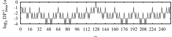
Fig. 2. Tabulation of values

}

cB CR5,

#Xâ

R

âßãã , for

þ

. For example, P

cB Jä"

þ

and}

cB

ãå

þ

5FA

that#S$_&`TU+V (+*4 is equal to the (more relevant for the DC) valueXbZc\ d;æ² o5#%$'&TU+Vc(^*_,O-4

whenever*n~8±u . Note that the naive algorithm for the same problem works in time

ç

(

¡

4 , which makes it practically infeasible even for8k i .

Theorem 5. For every*Ù¬Y§ , Algorithm 5 computes#%$'&` TU+V (+*4 in timev[(DwBx>y_p4 .

Proof (Sketch). By the same arguments as in the proof of previous theorem, given inputs

(^*_,.*M4, the value2M68*×JQ(- 4 (^*_,.*M4pº ÎSÏÐÑ

(D¯µ 4O4 is(^*_,.*M4-optimal. We now prove

by contradiction that #%$ &` TU+V (^*M4t8ª#%$ &TU+V (+*', *4. Let - ~8ª* and 20K be such that

#S$ & (^*_,O-0/1320KB4N #S$ &TU+V (^*_,.*M4. By Algorithms 2 and 4, there is an ´üáµm

such that ÆÇ(+*',.-|,20KB4O®L8 and -64l(^*_,.*M4®L8ª . But then, on the other hand, since

the differential (^*_,O-æ/1 2;K4 is possible and -64l(^*_,.*M4®À8ö , it is also the case that

ÆÇ(^*_,O-|,O2;K4®

8èu . Since -64>(+*', *4O®8 YÉè-64>(+*', *4O®

8åu , we have also that

-64>(^*_,.*M4®

8¸u . Therefore#S$ & (^*_,O-0/1320KB4ñ#%$ &TU+V(+*',*4.

Straightforwardly, Theorem 5 helps to find many interesting properties of#%$ &` TU+V. For

example, #%$ &` TU+V (^*M4b83 iff*tºH(+A µ 4[8nu , andX8é^ê

#%$ &` TU+V (^*M4b8±e ¹.

. Another consequence is that#S$'&` TU+V (+*4 8

iff (1)

*Yº(e µQ 48 µëñEK for

someu´ìYüg , or (2)*Yº(e µQ 48æë for someu´íìü½tµQ . For better

understanding, all values of#S$ &` TU+V (+*4,8¸f , are depicted in Fig. 2.

Once again, our results may be compared with the results in [O’C93,O’C95] that

show that for an -bit permutation (resp. composite permutation, controlled by an

-bit string) the expected probability of the maximum nonzero differential is Á>e

(resp.

º

).

Further Work and Acknowledgments

While we leave practical applications of our results as an open question, we note that our results have already been used in [MY00] for truncated differential cryptanalysis of Twofish.

The current work bases somewhat on [Mor00], that had a (correct) linear-time

al-gorithm for #%$'& , but with an incorrect proof. We would like to thank Eli Biham for

(15)

References

[AKM98] Kazumaro Aoki, Kunio Kobayashi, and Shiho Moriai. The Best Differential Charac-teristic Search of FEAL. IEICE Trans. Fundamentals, E81-A(1):98–104, January 1998. [Ber92] Thomas A. Berson. Differential Cryptanalysis Mod

¢

with Applications to MD5. In Ernest F. Brickell, editor, Advances in Cryptology—CRYPTO ’92, volume 740 of Lecture

Notes in Computer Science, pages 71–80. Springer-Verlag, 1993, 16–20 August 1992.

[BS91a] Eli Biham and Adi Shamir. Differential Cryptanalysis of DES-like Cryptosystems.

Journal of Cryptology, 4(1):3–72, 1991.

[BS91b] Eli Biham and Adi Shamir. Differential Cryptanalysis of Feal and N-Hash. In Don-ald W. Davies, editor, Advances on Cryptology — EUROCRYPT ’91, volume 547 of

Lecture Notes in Computer Science, pages 1–16, Brighton, UK, April 1991.

Springer-Verlag. Full version available from

http://www.cs.technion.ac.il/˜biham/, as of April 2001.

[Dae95] Joan Daemen. Cipher and Hash Function Design. Strategies based on linear and

dif-ferential cryptanalysis. PhD thesis, Katholieke Universiteit Leuven, 1995.

[DGV93] Joan Daemen, Ren´e Govaerts, and Joos Vandewalle. Cryptanalysis of 2.5 Rounds of IDEA. Technical Report 1, ESAT-COSIC, 1993.

[Knu99] Lars Knudsen. Some Thoughts on the AES Process. Public Comment to the AES First Round, 15 April 1999. Available from

http://www.ii.uib.no/˜larsr/serpent/, as of April 2001.

[LMM91] Xuejia Lai, James L. Massey, and Sean Murphy. Markov Ciphers and Differential Cryptanalysis. In Donald W. Davies, editor, Advances on Cryptology — EUROCRYPT

’91, volume 547 of Lecture Notes in Computer Science, pages 17–38, Brighton, UK,

April 1991. Springer-Verlag.

[Miy98] Hiroshi Miyano. Addend Dependency of Differential/Linear Probability of Addition.

IEICE Trans. Fundamentals, E81-A(1):106–109, January 1998.

[Mor00] Shiho Moriai. Cryptanalysis of Twofish (I). In The Symposium on Cryptography and

Information Security, Okinawa, Japan, 26–28 January 2000. In Japanese.

[MY00] Shiho Moriai and Yiqun Lisa Yin. Cryptanalysis of Twofish (II). Technical report, IEICE, ISEC2000-38, July 2000.

[NK95] Kaisa Nyberg and Lars Knudsen. Provable Security Against a Differential Attack.

Jour-nal of Cryptology, 8(1):27–37, 1995.

[O’C93] Luke J. O’Connor. On the Distribution of Characteristics in Composite Permutations. In Douglas R. Stinson, editor, Advances on Cryptology — CRYPTO ’93, volume 773 of

Lecture Notes in Computer Science, pages 403–412, Santa Barbara, USA, August 1993.

Springer-Verlag.

[O’C95] Luke O’Connor. On the Distribution of Characteristics in Bijective Mappings. Journal