Three Essays on the Welfare Effects of Organic Milk Introduction.

ABSTRACT

CHOI, HEE JUNG. Three Essays on the Welfare Effects of Organic Milk Introduction. (Under the direction of Dr. Michael Wohlgenant.)

This study investigates the impact of organic milk introduction on consumer benefits employing two different demand approaches; multistage demand system approach and discrete choice approach. These two approaches with A.C. Nielsen Homescan data allow analyzing the dairy market at the various levels of the economy.

In the first essay, the aggregate demands for milk products at both brand level and commodity group level are analyzed adopting the multistage demand system approach. Expenditure functions are derived from the estimated demand equations to quantify the welfare changes. The welfare effect is decomposed into the variety effect and the price effect, where the former is the willingness-to-pay changes for having more options to choose and the latter is the amount of price changes in existing products due to enhanced competition. Unlike the previous demand studies on milk market, the elasticity results indicate that there is no evidence of substitutability between organic and conventional milk products when milk is categorized by both fat contents and organic claims. Rather, this study shows that milk products with similar fat content are substitutable to each other. The estimated variety effects indicate that consumers benefit significantly from the organic option as much as 8% of milk expenditure. The price effects show some evidence of cannibalization in this market over the period of analysis.

that households with younger head, higher income and higher education benefit more from organic milk introduction than ones with older head and lower income and education.

Three Essays on the Welfare Effects of Organic Milk Introduction

by Hee Jung Choi

A dissertation submitted to the Graduate Faculty of North Carolina State University

in partial fulfillment of the requirements for the Degree of

Doctor of Philosophy

Economics

Raleigh, North Carolina 2011

APPROVED BY:

_______________________________ ______________________________ Michael Wohlgenant Atsushi Inoue

Committee Chair

DEDICATION

BIOGRAPHY

ACKNOWLEDGMENTS

There are a lot of individuals who have been helping me on the bumpy road of pursuing a Ph.D. A few words here cannot express my gratitude to them of making this possible. I would first recognize my advisor, Dr. Michael Wohlgenant, for his patience, guidance and never-ending encouragement. Every Friday afternoon with him was full of valuable discussions on various issues from the ones addressed in this dissertation to personal beliefs and philosophies on teaching and research. Independent thinking and self-motivation that he taught me will be valuable assets as I pursue my career.

I also express sincere appreciation to Dr. Xiaoyong Zheng for being supportive all the time. His comments and down-to-earth inputs were exceptionally helpful to overcome various obstacles. Special thanks to Drs. Nick Piggott and Atsushi Inoue for their insightful comments and corrections, and to Dr. Tamah Morant for all the departmental supports that allowed me to focus on my research and study. I also would like to thank my former supervisor at Korea Development Institute, Dr. Hyun-Wook Kim, for encouraging me to start a Ph.D.

I thank my friends in the department especially Yudis, Takahiro, Tim, Joe, Steve and Xiaofang who made my graduate years bearable and interesting. Special thanks to my friend Yu-Jeong Choi for her prayers and encouragements.

The very deepest thanks go to my parents who are the biggest influence in my life. Their unceasing love and faith gave me courage and strength whenever I fell down. I have never felt in needs because of their prayers and tears as well as financial supports. I also thank my generous husband, Dr. Sung Hong, for his love and support and my dear brother, Jae Choi, for being always there for me.

TABLE OF CONTENTS

LIST OF TABLES ... vii

CHAPTER 1 ... 1

The Welfare Effect of Organic Milk ... 1

I. Introduction ... 1

II. Demand Estimation for Differential Goods ... 5

1) Classical Approach ... 6

2) Logit Approach ... 7

3) Multi-stage Demand ... 8

III. Data ... 9

IV. Model ... 12

1) Multi Stage Demand System ... 12

2) Specification and Estimation ... 14

V. Welfare Analysis ... 20

VI. Results ... 23

1) Elasticity Estimates ... 23

2) Variety Effects... 25

3) Price Effects ... 26

VII. Conclusions ... 27

REFERENCES ... 28

CHAPTER 2 ... 40

Household Level Welfare Effect of Organic Milk Introduction ... 40

I. Introduction ... 40

II. Literature Review... 42

1) Discrete Choice Models ... 42

2) Demand for Differentiated Goods and Welfare Studies ... 44

1) Random Utility ... 46

2) Choice Probabilities ... 48

3) Elasticities ... 49

4) Welfare Analysis ... 50

IV. Data and Estimation ... 51

1) Data ... 51

2) Estimation... 53

V. Results ... 55

VI. Conclusions ... 59

REFERENCES ... 61

CHAPTER 3 ... 76

The Competitive Effects of Organic Milk Introduction ... 76

I. Introduction ... 76

II. Fluid Milk Industry ... 78

III. Model ... 80

1) Supply and Equilibrium ... 80

2) Consumer Welfare... 81

IV. Estimation... 83

1) Discrete choice model ... 83

2) Multi-stage Demand model ... 86

V. Results ... 88

VI. Conclusion ... 90

LIST OF TABLES

Table I- 1 Distributions of Observed Household Attributes in the US ... 30

Table I-1 Continued ... 31

Table I- 2 Market Shares of Organic and Non-organic Milk by Observed Demographic Attributes at the National Level ... 32

Table I- 2 Continued ... 33

Table I- 3 Market Shares by Fat Contents and Organic Claim in the US ... 34

Table I- 4 Market Share by Fat Contents and Organic Claim in RDU ... 34

Table I- 5 Summary of Commodity Groups in RDU ... 35

Table I- 6 Conditional Elasticities at the Group Level with Time Trend ... 36

Table I- 7 Unconditional Elasticities with time trend ... 37

Table I- 8 Unconditional Elasticities at the Brand Level ... 38

Table I- 9 Variety Effects ... 39

Table I- 10 Price Effects ... 39

Table II- 1 List of Products in the Choice Set ... 64

Table II- 1 Continued ... 65

Table II- 2 Market Shares by Size and Fat of Products ... 66

Table II- 3 Descriptive Statistics for Observed Household Attributes ... 66

Table II- 4 Parameter Estimates from the Mixed Logit Model ... 67

Table II- 5 Elasticity Estimates from the Mixed Logit Model... 68

Table II- 5 Continued ... 69

Table II- 5 Continued ... 70

Table II- 5 Contined ... 71

Table II- 5 Continued ... 72

Table II- 6 Elasticities at the Group Level ... 73

Table II- 7 Distribution of Variety Effect by Age ... 73

Table II- 8 Distribution of Variety Effect by Education ... 74

Table II- 9 Distribution of Variety Effect by Income ... 74

CHAPTER 1

The Welfare Effect of Organic Milk

I. Introduction

Recent innovations in agricultural industry make new products, such as Genetically Modified (GM) food and Organic food, available to consumers. Although various opinions on the effect of GM food products are not in agreement among nutrition experts, consumers‟ concern on health and environment increases demand for organic food products. This study analyses the structural changes driven by organic food introduction into the U.S. food sector in terms of its welfare effect. According to the Organic Trade Association (OTA), organic food sales in the U.S. were $13.8 billion in 2005, which is 2.5% of total food sales. This is an increase from 1.9% in 2003 and from 0.8% in 1997. Increasing trends of demand are expected to continue and estimated to rise to $23.8 billion by 2010 (Nutrition Business Journal, 2004). Public policy also played a significant role in the expansion of organic food sector. The National Organic Standards, which is implemented by the U.S. Department of Agriculture (USDA) in 2002, specify the production process for processing, distributing, and growing organic food. The policy also restricts the use of Organic logo by allowing it only to the products whose profile meets the standards. Consumers are not only exposed to more information on organic standard by this policy adoption, but the logo also provides an easy way for consumers to recognize qualified organic products.

market, sales of organic milk have been growing; organic milk and cream sales increased from $15.8 million to $104 million, from 1996 to 2000. The industry shows a dramatic increase in sales during the early 2000s, which coincides with the implementation of National Organic Standards1 in 2002 and a price increase of conventional milk in 2004. As of 2005, organic milk and cream sales were over $1billion, which is 25% up from 2004 sales. A noticeable fact is that overall sales of milk have remained constant since the mid-1980s, which indicates that organic milk sales not only increased, but also expanded in its market share in overall milk industry (Miller and Blayhey, 2006). This also implies that not only new firms entered the organic milk industry during the past years, but also existing firms increased the supply of organic milk by recruiting and assisting conventional milk producers converting their product to organic milk2. (USDA, Retail and Consumer Aspects of the Organic Milk Market)

As interest in organic market grow, agricultural researchers have conducted some studies on organic milk. An earlier study by Glaser and Thompson (2000) considers demand for branded milk, private label milk and organic milk based on supermarket scanned data collected from 1988 to 1999 by AC Nielsen and Information Resources, Inc (IRI). According to the study, demand elasticities computed from nonlinear Almost Ideal Demand System (AIDS) framework indicate that organic milk demand is more elastic than private-label and branded milk. Although this analysis well describes the sensitivity of organic milk demand in the early stages of introduction, it cannot account for the current market analysis because the

1

Organic dairy products, as defined by USDA, are made from the milk of animals raised organic management. The animals are raised separately from the herd of conventional dairy animals. The animals are not given hormones or antibiotics. The animals receive preventive medical care, such as vaccines, and dietary supplements of vitamins and minerals. (Recent Growth Patterns in the U.S. Organic Foods Market, USDA)

2

organic market has grown competitive to the extent that private label milk suppliers also produce organic milk.

The type of consumer more likely to purchase organic products has also been of interest to marketing researchers. Lohr (2001) characterizes organic consumers as White, affluent and well-educated. Lohr and Semali (2000) conclude that parents of young children or infants are more likely than those without children to purchase organic food. Dimitri and Venezia (2007) provide descriptive statistics on the socio demographic characteristics of organic milk consumers using 2004 Nielsen Homescan panel. They also conclude that the typical organic milk consumer is white, well-educated and living in a household headed by someone younger than 50 years old, which is not different from the description on general organic consumers studied by others. Alviola and Capps (2008) provide a more formal statistical analysis with the same data as Dimitri et al. implementing Heckman two-step procedure. Their conclusion largely agrees with Dimitri et al.

mentioned above, the National Organic Standards, as well as many media reports on health issues, contributed to changing consumers‟ perception of organic milk. Hence, it is very likely that consumption patterns on organic and conventional milk changed after this policy. This idea can be supported by the report that more consumers have bought the higher premium especially after 2002 (Dimitri et al, 2005). Consumers‟ concern on health risk and retailers‟ response also changed the structure of milk market. The nation‟s largest diary process, Dean Foods, no longer sells rBST treated milk, and the top 3 grocery retailers, Wal-Mart, Kroger, and Costco, claimed not to sell such milk in their stores. Therefore, rBST treated milk is not in the product space for most of consumers after the early 2000s; hence, the categorization used in their study will not be valid any longer. Second, the model does not control other relevant factors such as fat contents or flavor. Based on the fact that consumers‟ preference on fat contents has been changed as their concerns on fat consumption increase, it is possible that this model over states the welfare effect of organic milk.

In the early stage of introduction of organic milk, there existed only two organic milk suppliers in the nation, Organic Valley and Horizon Organic, and they were available in some limited areas. Thus, the structure of competition in milk market is rather between organic milk and non organic milk. As the organic milk market has expanded, however, the competitive structure has also changed to the extent that there are several national and local brand organic milk plus private-labeled organic milk carried by conventional supermarkets. Therefore, in order to establish an appropriate analysis of current milk market, the competition at the brand level rather than commodity group level should be taken account into the model.

data from 2004 to 2005 is used for the study3. The multi-stage demand approach is used to estimate the demand for milk products at the brand level following Hausman (1997). The Linear Approximate AIDS (LA/AIDS) model is adopted for the functional form of demand equations. Unconditional (on the expenditure) elasticities among brands and group commodities are estimated using the methodology suggested by Carpentier et al.(2001). In addition, the welfare effect of the introduction of organic milk will be analyzed.

Previous studies on brand level demand analysis are reviewed in section II and descriptive statistics from Nielsen Homescan data are presented in section III. Section IV explains model specification and estimation techniques for demand analysis and the results are shown in section V, and the welfare analysis is provided in section VI.

II. Demand Estimation for Differential Goods

Researchers have been interested in developing methodologies to estimate demands for differentiated goods as disaggregated data and advanced computational devices have become available. For example, Hausman et al. (1994) proposed a multi-stage demand system with an application to beer market and Berry et al. (1995) introduced mixed logit approach with an application to automobile demand. Although the applications to differentiated goods and disaggregate data are recent innovations, their basic ideas are from the existing demand approaches. In this sense, the development of classical demand approaches is briefly discussed and two representative demand approaches in differentiated goods context are discussed.

3

1) Classical Approach

Since Stone (1954) derived the very first demand system, Linear Expenditure System (LES), by imposing theoretical restrictions on a simple linear demand system, researchers have developed various functional forms of demand equations to reflect the reality better so that be able to test whether the theoretical restrictions are true. Theil (1965) and Barton (1966) derived Rotterdam model (RM) by substituting Slutsky decomposition into a differentiated double log demand function. Homogeneity, symmetry and negativity are tested, but Barton finds that the empirical results of RM are consistent with theory only with the application to highly aggregated data while disaggregated applications conflict with theory. Different approaches that give more functional flexibility to the model were suggested by a great number of researchers in order to find a model consistent with theory. The basic idea of flexible functional forms is to approximate direct utility function, indirect utility function or cost function by some specific functional forms and give it enough parameters so that it is flexible enough to approximate an arbitrary utility or cost function. The demand functions are derived through duality. Christensen, Jorgenson, and Lau (1975)‟s translog model approximates the indirect utility function by a quadratic function of logs of normalized prices, and derive Marshallian demand by Roy‟s identity. The authors also test theoretical restrictions, but homogeneity does not hold for this model. Another famous approach known as Almost Ideal Demand System (AIDS) is introduced by Deaton and Muellbauer (1980). The model is derived from the cost function of generalized Gorman polar form using Shephard‟s lemma. The test with this model is also inconsistent with theoretical restrictions.

not hold. But most researchers, such as Deaton and Muellbauer, carefully conclude that none of the existing models perfectly define demands and measure elasticies, and estimate the best approximation imposing the theoretical restriction.

2) Logit Approach

McFadden (1974) argues that the conventional demand approach assumes all individuals in a population have a common behavioral rule. The logit model starts from the indirect utility functions of individuals instead of a “representative” utility, taking account heterogeneity of individual tastes. The indirect utility function consists of common utility and random utility. Based on the revealed preference theory, probability of choice can be presented as an integral of cumulated joint density functions. This probability directly can be interpreted as the share of demand, but it has to be transformed into a closed form of a function for estimation purpose. Luce (1956) derived the probability of choice formula from the conditions satisfies Independence of Irrelevant Alternative (IIA). McFadden (1974) derived the same probability of choice formula under the assumption of Gumbel distribution for the error terms.

A nice feature of logit models is that the tastes that vary systematically with respect to observed variables can be captured while the tastes that vary with unobserved variables cannot be handled. Also, the logit models solve the problem of having large number of parameters which conventional demand system suffers from because the indirect utility functions in discrete choice model are not defined with the prices of all the products in the system. However, the substitutability in logit models is very restrictive. Since logit models exhibit the independence of irrelevant alternatives (IIA) property, it constrains the cross price elasticities. The IIA claims that the ratio of choice probabilities between two goods does not change even if the third irrelevant good is introduced. This might be a plausible assumption in some cases, but it is not behaviorally accurate in many cases.

decisions in sequence. Consumers would choose whether to participate in the economic activity in question, then select a specific choice. Within each data step, the IIA assumption holds. However, across different steps, the ratio of probabilities can depend on the attributes of other alternatives in those nests and IIA does not hold. Nested logit approach is still limited in its ability to account for unobserved preferences. To relax the IIA assumption and account for heterogeneity, the mixed logit model is used (Train et al. 1987 and Berry 1995). It is an extension of standard logit that allows the coefficients to vary across individuals by assuming the coefficients have distributions rather than fixed numbers.

3) Multi-stage Demand

Hausman et al.(1994, 2002) apply Gorman‟s multi-stage budgeting approach into the demand for differentiated products. Strotz (1957) discussed that consumers allocate expenditure among broad groups of commodities in the first stage of budgeting, and then allocate individual commodities within each group if the utility function is separable. Gorman (1959, 1971) developed Strotz‟s discussion in detail. He argues that „separability‟ is not enough to explain the consumer‟s multi-stage budgeting behavior. He shows that, under the assumption of „weak separability‟, consumers allocate their income into broad groups of commodities at higher stage of budgeting and more detailed within-group allocation happens at lower stage. Weakly separable preferences allow the last stage demand functions to be presented only with the group expenditure and the prices of products within that group. However, in order for the higher stage demand functions to be expressed with total expenditure and the price indices of each group, additive separability and Gorman generalized polar form of indirect utility functions, or homothetic preference is required.

of demand equations suffered from its numerous coefficients to estimate. Weak separability is assumed at the lowest level of utility maximization problem so that the demand for each brand can be presented as a function of group expenditure and the prices of own and other brands in the same group. Additive separability is required at the higher stage of utility maximization in order for the higher stage demand to be presented as a function of total beer expenditure and price indices of segments. Although additive separability has nice features which reduces the number of coefficients allowing the demand function to be written with group price and quantity indices instead of commodity prices, it is not a realistic nor plausible assumption. Hausman does not explicitly discuss the assumptions for the higher stage demand, but it seems that he adopts Carpentier and Guyomard‟s (2001) approximation of first-stage allocation process instead of imposing additive separability. Carpentier states that, if preferences are weakly separable and the group price indices being used do not vary too greatly with the utility level, allocation between groups of commodities by two stage budgeting will be consistent with unconditional demand analysis, thus the first stage demand function with price index can be approximately rationalized without a strong assumption.

III. Data

As mentioned above, the data used in this study are the Nielsen Homescan panel data. The sample is selected among volunteers based on both demographic and geographic targets. Stratification is done by AC Nielsen to ensure that the sample matches the U.S. Census. The panelist members are required to scan the items purchased with handheld scanner and transfer the information to AC Nielsen each week identifying purchase date. Unobserved data should be interpreted as infrequency of sales rather than infrequency of records since it is mandatory for the members to transfer data every week. If a member fails to comply with the rule and does not report more than a month, then the panelist membership is terminated.

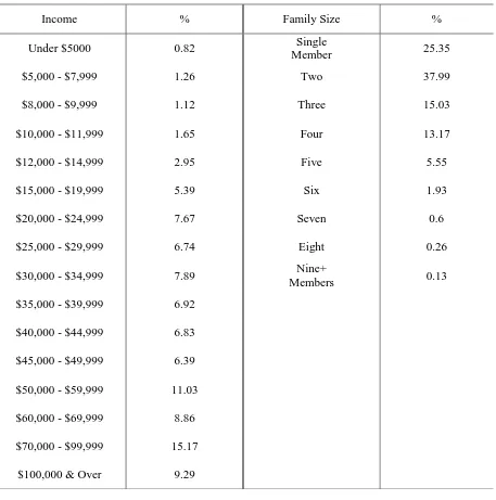
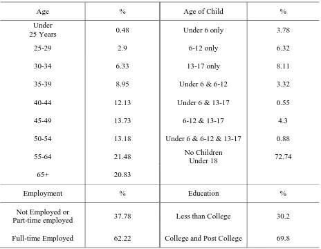
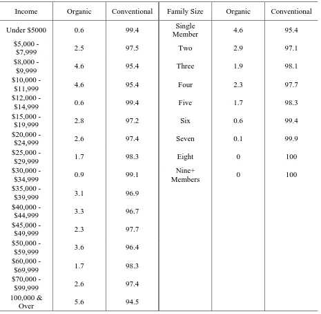
sample contains information on demographics such as income, household size, age of head, number of child, employment, education and race. Demographic distributions are presented in TableI-1. Half of the sample is from under $45,000 income class and the other half is from above $45,000 income class. More than half of the households consist of single or two members, and 75 percent of the sample have no children under 18. 72 percent of male or female household heads are employed more than 30 hours a week and 70 percent of them have at least college degree. The shares of organic milk purchase by different demographic characteristics are provided in Table I-2. Households with small number of members tend to purchase more organic milk than large families do. Middle income class is less likely to purchase organic milk than low income or high income class. Also, the data show that the households only with under-6-year-old children are relatively more likely to purchase organic milk than any other households.

A number of physical product characteristics, weekly prices and quantities purchased are also included in the data. For simplicity, milk products are differentiated with a few important characteristics such as fat contents, flavor and organic claim4. The fat contents are categorized into five types in this study; non-fat, 1% low fat, 2% reduced fat, whole milk and soy&lactose-free milk. Flavor is categorized into flavored and not flavored. Table I-3 provides the market shares of products distinguished by these characteristics each year. 2% reduced fat milk brings the largest share of milk sales up to 35% during the period, and the market shares of 2% milk and whole milk have decreasing trends while the shares of non-fat, low fat and soy&lactose-free milk have moderately increasing trends. The share of organic milk also shows an increasing trend in this sample.

In this study, a product is defined at the brand level with four different characteristics of products; fat contents, organic claim, flavored or not and the name of manufacturer. Many kinds of flavors are consolidated into “flavored” for simplicity. Different fat contents produced by the same manufacturer are treated as different products, and organic milk and

4

non-organic milk of a same producer are treated as different products as well. Different brands with same fat contents, flavor and the same organic claim are, of course, regarded as different products. But different sizes and different types of containers are not distinguished in the products defined in this study. The commodity groups are aggregated across different brands with the same characteristics. For example, the commodity group of 2% reduced fat-organic-unflavored milk is an aggregation of different brand names within the group of 2% reduced fat-organic-unflavored milk. Hence, there are 20 group commodities with the categorization mentioned above. The quantities of group commodities are the aggregation across brand level products with same characteristics and their prices are the price indices of each group. In terms of time frequency, weekly purchase data are aggregated into monthly records in order to minimize infrequency problem. According to the definition of product above, there exist 1,902 products in the nation. However, it is notable that specific brands of milk appear only in specific areas and only a few brands dominate the local markets while a large number of residuals take only 1~5% of market share. Hence, it is concluded that the brand-level milk market is highly localized and dominated by a few brands so this study needs to focus on some specific market. Raleigh-Durham-Chapel hill and Charlotte markets are chosen and brands with market share larger than 1% are considered.

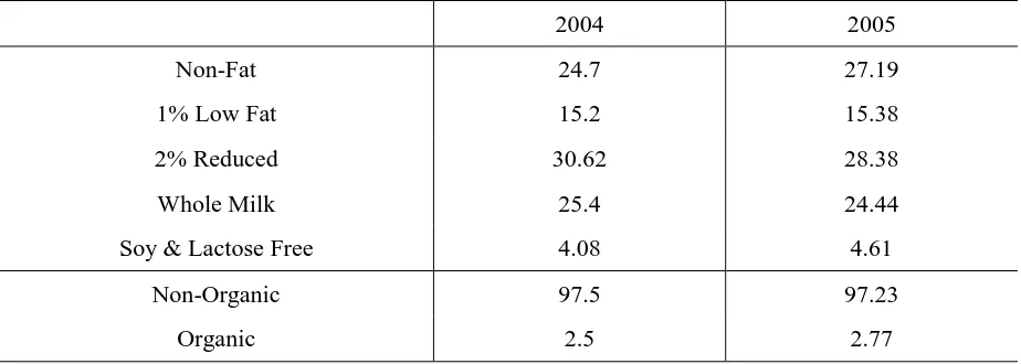
assumption that organic cow milk is introduced in this area since 2004. The price values of conventional milk prior to 2004 are used to calculate the price effects in the welfare analysis. The shares of each type of milk sales are described in Table I-4. The figures are similar to the national sample. The organic milk takes about 2.5 percent of the milk market and the 2% reduced fat milk takes the largest share.

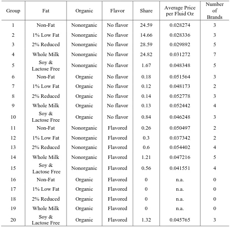
There exist 249 products in the area, but only 58 products take more than 97% of the milk market. Hence, only the 58 products are included in this study. The products can be categorized into 20 groups according to the characteristics mentioned above, which are fat contents, flavor and organic claim. Market shares and average prices of products in each group, and the number of brands with larger than 1% of market share within each group are shown in Table I-5. Conventional non-flavored non-organic milk dominates the market with 92% market share. Soy and lactose free milks are priced higher than cow milk among non organic milk. Organic cow milk has higher per unit prices than conventional cow milk as expected, but soy and lactose free milk are not priced differently between organic and non organic.

IV. Model

1) Multi Stage Demand System

level demand equation is specified as Linear Approximate Almost Ideal Demand System (LA/AIDS):

(1)

 

i j G i j n

P m p w _it G t G t i n j jt ij it

it ln ln , , , , 1,2,...,

1            



    

where i1,2,...,n denotes the brands of milk in group G and t denotes time period. p_jt are the price of product j consumers face in time period t. m_tGare total group expenditure on

group G in period t, that is,



  n i it it G

t p q

m

1

and it is an error term. G t

P is the Linear

Approximate AIDS price index of brands in group G period t.

In order to estimate the group commodity demand in the second stage, Stone Index is computed for the price indices of each segment using mean values of market shares of each brand. LA/AIDS is used to specify the middle level equation. (Hausman states in his paper that the difference in functional form does not make difference in outcomes.)

(2) _mt M k kt ij B t Bt m mt e P y

q  





1

log

log  



m = 1, …, M, t = 1, …, T

where q_mt is the share of segment m in period t, y_Btis total milk expenditure, and π_kt is segment price indices in the period of t.

The first level equation, which explains the overall demand for milk, can be specified as

(3) logu_t ₀ ₁logy_t ₂log_t Z_t e_t

where ut is overall consumption of milk, yt is disposable income, πt is price index for milk,

2) Specification and Estimation

As I mentioned above, data used in this study are micro-level survey data. When it comes to demand analysis using this type of data, one cannot avoid the issue that some products are not consumed by at least some economic agents in some periods. Even though the data used in this study for the lower level of multistage demand equation are not disaggregated as to the household level, the data are still disaggregated to some degree of brand level and indicate zero purchases for some brands in some periods.

Setting aside the difficulties of estimating latent dependent variable models, missing regressor difficulties are first encountered because prices are not observed for non purchased products. Three simple solutions for this problem are 1) to discard all incomplete observations and estimate population parameters using the remaining observations, 2) to use zero-order methods which substitute sample means for the missing values, and 3) to use first-order methods which substitute predicted values from simple regression for the missing values. However, these methods are criticized because of sample selection bias. Many researchers suggest various missing value procedures mostly utilizing demographic or product characteristics. For example, Heckman procedure and Amemiya‟s principle require both regressands and regressors in demand systems to be endogenous so that the variability of regressors can be explained with other exogenous variables. However, in multi-stage demand approach, it is difficult to incorporate quality adjusting price equations because the assumption of separability does not allow volatilities in the exogenous variables that explain price variation, such as characteristics of products. Therefore, a simple regression method seems to be the only feasible approach to treat the missing price problems. The unobserved unit prices are predicted following Perali and Chavas (2000). The unit prices at UPC level were regressed on characteristics variables, time variables, regional dummies, and interaction terms between characteristics and time variables. The least square results show 0.54 of R-square, but the coefficient estimates are statistically significant at 10% level.

outcomes of consumer utility maximization problem, which are rational decisions of economic agents. Thus, a Tobit model is suggested to explain the corner solutions.

           0 0 0 * * * it it it it w if w if w w

Assuming random utility hypothesis (RUH) and PIGLOG class utility function, the Marshallian uncompensated demand functions at the household level can be specified as follows:

(4)

 

i j G i j n

P m p w _iht G ht G ht i n j jht ij iht

iht , , , , 1,2,...,

~ ln ln 1 *            



    

where i1,2,...,n denotes the i ‟s milk product in the demand system, h denotes the household, t denotes the time period. p_jht is the price of product j household h faces in time period t. m_htis household h‟s total group expenditure on milk products in period t,

that is,



  n i iht iht G

ht p q m

1

and G ht

P is the Linear Approximate AIDS price index for household

h in period t. ~ is an error term that is heteroskedastic within the share equation for one iht good and correlated across the share equations for different goods.





 iht i _j jht jht

iht   p 

~ ln . _jht is mean zero homoskedastic error term from utility function.

(5)





    T t iht ih n i iht ih G ht w T w p w P 1 0 1 0 1 where ) log( log .

Household heterogeneity _iht might be specified as

(6) _{kht i s is h}

s k

ik i

iht   d   t  t c





2 ) 2 ( ) 1 ( 1

0   

 

(7)

 

i j G i j n P

m p

w _{G it}

t G t i n j jt ij it

it , , , , 1,2,...,

~ ln ln 1 *            



     where 2 2 1 0 * , ~ ~

, t t

m m

m w m

w _{it i i i}

h G ht h iht G ht it h ht h iht ht

it    

      









Therefore, heteroskedastic Tobit model with the two-step estimation approach is adopted for the lower stage demand estimation.

The first and the second stage demand do not require Tobit approach because the aggregated data used in the higher stage do not show the evidence of corner solution outcomes. However, the error terms might not be homoskedastic any longer. Based on the assumption of Random Utility Hypothesis, disturbances of uncompensated demand functions will be heteroskedastic according to the same logic provided above. Hence, the conventional demand systems given in equation (2) and (3) with SUR approach are adopted for the higher stage demand estimation.

Two step estimation

Meyerhoefer, Ranney and Sahn (2005). This study adopts Meyerhoefer‟s two-step estimation because the approach is generalized to the application of panel data while others are applied only with cross-section data and its computational procedure is relatively simple comparing to other approaches.

The basic idea of the two-stage procedure is to estimate an unrestricted heteroskedastic Tobit model equation by equation and find the error correlations, and then recover restricted parameters using the minimum distance method which falls into the GMM framework.

In the first step, the share equation for ith product presented by equation (7) can be rewritten as follow if time variables are dropped.

(8)

 

i j G i j n

P m p w _it G t G t i n j jt ij i

it , , , , 1,2,...,

~ ln ln 1 0 * _{  }         



    

where







 

 iht iht i _j jht jht

h G ht h iht G ht it p m m     

 , ~ ln

~

~ _.

0

i

 is product specific fixed effect. As ~ is heteroscedastic within each equation _iht and correlated across equations, so is ~ . To get consistent first-step estimates, a _it heteroscedastic Tobit econometric model is employed for each equation. The variance of the error term is specified using a fairly flexible and general form

(9) Var(~_it)_i2exp

 

z_it'_i

where zit is a sz-dimensional vector of variables for product i in period t. Variables of t,

2

t , log pit and _G t

G t P m

log were included in zit at first, but only _G t

G t P m

log is included because the

obtain from this step are reduced form estimates. In order to recover restricted estimates,

reduced form parameter estimates are collected in the vector

' ' '

1,..., 

         n  

 , where



i

 is a



ns_z 2



1 vector of reduced form parameter estimates from the i‟s equation. In the

second step of estimation, the cross equation restrictions implied from demand theory are imposed on the reduced form parameters estimated in the first step, and the structural parameters that are consistent with demand theory are calculated. Denote a q-dimensional vector of structural parameters as  , then the structural parameters are obtained from the following GMM estimation procedure

(10)              ) ( ) ( min 1 '    

 h h

where h() is a nonlinear mapping  into  that is used to impose the theoretical restrictions on the reduced form parameters. The number of restrictions imposed is



ns_z 2



nq, which is equal to (n-1)*n/2+n+2. Under the null hypothesis that these restrictions are correct, the minimized value of objective function (10) is a chi-square distributed random variable with degree of freedom equals to the number of observation minus the number of restrictions.

The difficulty arises in finding a consistent estimate of . Meyerhoefer et al. (2005) states that the covariance-variance matrix for



 takes the form 2 11 1 1

 



 D D D and the proof

is provided in his unpublished dissertation (2002). If gt 



g1't,...,g'nt



' denotes the vector of univariate scores from all of the n equations corresponding to the observation in period t, and H_it the univariate Hessian from the i ‟s equation for the same observation, then

 

 



1 1



1 1 1 ,...,    _ nt

t E H

H E diag

observations for each brand is at most 24. The data for specific types of milk such as organic milk are established recently, thus very short strings of data are available for special types of milk.

The finite sample properties of GMM estimator seem to be an interesting topic among the econometricians in mid 90s. The July 1996 issue of Journal of Business and Economic Statistics is full of papers on the small sample properties of GMM estimator proposing alternatives for consistent estimator of weighting matrix. Although they are looking at slightly different issues of small sample properties, their conclusions converge to one that the equally weighted matrix, which is equivalent to identity matrix, dominates covariance matrix (or the proposed matrix) in terms of the bias of estimator and coverage probabilities. Therefore, the identity matrix is used in this study.

Elasticities

The unconditional expectation for the budget shares including all the observations is

(11)

 

 



 



 



                   



 iG i it i i

G i i n j jt ij i i it z P m p w

E    2 ' 

1

0 ln ln exp

) (

where

 

 

t i i G i G i i n j jt ij i z P m p      ' 2 1 0 exp ln ln                  





The uncompensated own price, cross price and expenditure elasticities that are conditional on the group expenditure but unconditional on whether the observed budget share is zero or positive can be derived as

(13)







 

 



) ( exp 2 1 ) ( ) ( ) ( 0 ' 2 0 it j i i ht i i j i ij i it it it it ijt w E w z w w E p p w E e                    where







 

 



) ( exp 2 1 ) ( 1 ' 2 it i ht i i i i i it w E z E           

The mean of elasticities over time are provided in the results section.



  T t ijt ij e T e 1 1

Unconditional (on expenditure) elasticities are computed following Carpentier and Guyomard (2001). The relationships between second-stage (i.e., conditional) and first-stage (i.e., unconditional) expenditure and price elasticities are established under the assumptions of weakly separable direct utility function and the approximate independence of the true cost of living indices with respect to sub-utility levels. Carpentier and Guyomard provide formulas with two-stage budgeting application, but the results are generalized to the three-stage budgeting application following Edgerton (1997).

V. Welfare Analysis

The total effect on consumers‟ welfare can be evaluated through compensating variation, which is the difference in consumers‟ expenditure function before and after the introduction of organic products holding utility constant at the post-introduction level:

(14) 𝐶𝑉 = 𝑒 𝑝₁, 𝑝_𝑁, 𝑟, 𝑢₁ − 𝑒(𝑝₀, 𝑝_𝑁∗(𝑝₀), 𝑟, 𝑢₁)

given the prices of other products. Following Hausman and Leonard (2002), this total benefit can be broken into two parts:

(15) 𝐶𝑉 = 𝑒 𝑝₁, 𝑝_𝑁, 𝑟, 𝑢₁ − 𝑒 𝑝₁, 𝑝_𝑁∗ 𝑝₁ , 𝑟, 𝑢₁ + [𝑒 𝑝₁, 𝑝_𝑁∗ 𝑝₁ , 𝑟, 𝑢₁ −

𝑒 𝑝0, 𝑝𝑁∗ 𝑝0 , 𝑟, 𝑢1 ]

and written as CV = −(VE + PE). The first term, variety effect (VE), represents the increase in consumer welfare due to the availability of the new products, holding the existing product prices constant at the post-introduction level. This effect not only captures the benefits from having more options but also the benefits from the new characteristics of new products. The second term, price effect (PE), represents the change of consumer welfare due to the change in the prices of existing products. The introduction of new products can lead the prices of existing products to increase or decrease depending on the competitive structure of the industry. If the new products closely compete with the existing products produced by the same manufacturer, the prices of existing products may rise. However, if the products compete closely with the existing products from different manufacturers, the prices of existing products are likely to decrease.

Price changes from the organic milk introduction are predicted at the group commodity level and the whole benefits in dollar values are measured at the aggregate level of milk industry using the price index of whole market. First, virtual prices can be evaluated at the group commodity level by solving a system of second level demand equations that would set the organic group commodities‟ shares to zero. There are 6 organic commodity groups among the total 16 commodity groups in this application. Given the virtual prices, variety effect can be calculated as follows:

(16) 𝑉𝐸 = 𝑒 𝑝₁, 𝑝_𝑁, 𝑟, 𝑢₁ − 𝑒 𝑝₁, 𝑝_𝑁∗ 𝑝₁ , 𝑟, 𝑢₁

The simplified expression can be integrated out and the indirect utility function can be obtained in a closed form by solving an ordinary differential equation. Finally, the corresponding expenditure function is obtained through inverting the indirect utility function. An explicit expression for the variety effect can be derived in case of a double log demand equation at the top level equation:

(17) 𝑉𝐸 = [ 1−𝛽1

1+𝛽2 𝑦1𝛽 1

𝑃 𝑝1, 𝑝𝑁∗ 𝑝1 𝑒𝑥𝑝 𝛿0+ 𝛽2𝑙𝑛𝑃 𝑝1, 𝑝𝑁∗ 𝑝1 − 𝑋1 + 𝑦11−𝛽1]

1 1−𝛽 1₋

𝑦₁

where p₁ and p_N∗ represent the post-introduction price indices for non organic commodity groups and the virtual price indices for organic commodity groups, respectively. Function P(∙) defines the virtual price index of the milk industry in this region. 𝛽1 is the coefficient on

log personal disposable income, 𝛽₂ is the coefficient on the milk price index from the top level equation, and 𝛿₀ captures the remainder of the variables in the top level equation. 𝑦₁ is post introduction personal disposable income and 𝑋1 is actual milk expenditure.

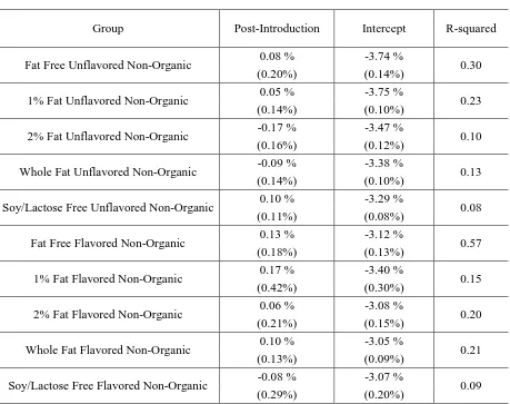
Hausman provides two different methodologies to estimate price effects. First, one can estimate the price effect directly from the data using OLS methodology if both the pre- and post-introduction consumption data for the existing goods are available. Second, one can estimate the price effects indirectly by solving the equilibrium conditions for the assumed model of competition for the post-introduction world. The price effects in this study are estimated with the direct estimation method because the interest of this study is on measuring the realized benefits without imposing any restrictions. The price effects are estimated with the following equation:

(18) 𝑙𝑜𝑔𝑝𝑖𝑡 = 𝛼𝑖+ 𝑊𝑡+ 𝐼𝑖𝑡𝛿 + 𝜀𝑖𝑡

of introduction is assumed to be 2004. For the price effect, the dataset is extended to 4 year periods. There are 48 months in the data and 47 dummies are included in the regression. 𝐼_𝑖𝑡 is a post-introduction indicator. 𝐼_𝑖𝑡 equal one if the organic milk is introduced. The coefficient 𝛿 measures the amount of price change of existing milk after the organic milk introduction5.

The overall effect of the organic milk introduction on consumer welfare is the sum of the variety effect and the price effect. Hausman (1981) derived the Compensating Variation in the same way he derived the Variety Effect:

(19) 𝐶𝑉 = [ 1−𝛽1

1+𝛽2 𝑦1𝛽 1

𝑃 𝑝₀, 𝑝_𝑁∗ _{𝑒𝑥𝑝 𝛿}

0+ 𝛽2𝑙𝑛𝑃 𝑝0, 𝑝𝑁∗ − 𝑋1 + 𝑦11−𝛽1]

1

1−𝛽 1_{− 𝑦1}

where P p₀, p_N∗ is the milk price index evaluated at the pre-introduction prices for the existing (conventional) milks and the virtual prices for organic types of milk.

VI. Results

1) Elasticity Estimates

I applied the econometric approach outlined above to the A.C. Nielsen Homescan data to estimate the system of milk demand equations. The estimates of equation (3), top level demand function, directly give the own price elasticity and the income elasticity, which are -0.2 and 0.88, respectively, in the RDU market. The milk price index in this market is calculated with the given data, the regional disposable income is indirectly obtained from Bureau of Economic Analysis (BEA) and Bureau of Labor Statistics (BLS).

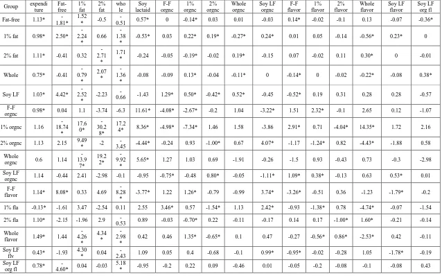
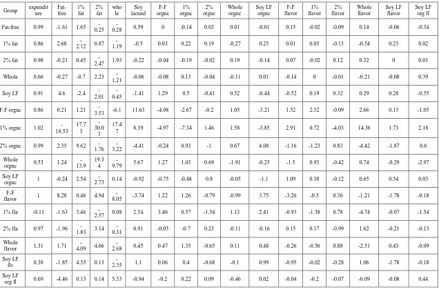
Elasticity estimates for the second stage demand system are provided from Table I-6 to Table I-7. The second stage demand equations are estimated both with and without the variables that account for time trend. The results partly conflict, but overall implications are not different between two models. Thus, the results with time trends are discussed in this

5

section because the model shows better fits. The value of minimization objective function is smaller and the number of significant estimates at 10% level is larger for the model with time trends. Table I-6 and Table I-7 show conditional and unconditional elasticity estimates, respectively. The elasticities are estimated at the mean of variables. Statistical significances are tested for the conditional elasticity and 108 estimates out of 272 are statistically significant at 10% level. The estimates are very similar between conditional and unconditional elasticities. Thus, the analysis provided below is based on the conditional elasticities because the significance tests are conducted for the conditional elasticities.6

All types of milk, except the organic-flavored soy/lactose free milk, show negative own price elasticities. Although the organic-flavored soy/lactose free milk has positive own price elasticity, it cannot be considered as Giffen goods because the estimate is not statistically significant. Cross price elasticities do not show a general pattern, but some implications can be drawn from the results. First, cross price elasticities between organic and conventional milk with same fat contents and flavor do not show a general pattern of substitution between organic and conventional milk. 1% fat unflavored organic and conventional milk have positive cross price elasticities (17.60 and 0.22) implying they are substitutes for each other, whereas organic and conventional unflavored whole milk have negative cross price elasticities (-9.92 and -0.11) suggesting that they are complements to each other. 2% fat milk and soy/lactose-free milk also have negative cross price elasticities between organic and conventional although they are not statistically significant. It is notable that the magnitude of substitution is not symmetric implying that the amount of organic milk consumption change when the conventional milk price changes is larger than the amount of conventional milk change when the organic milk price changes. Second, cross price elasticities show possible substitution patterns between fat contents although it is hard to conclude that similar fat contents are always substitutes with one another. Within the group of conventional unflavored milk, cross price elasticities show pretty clear substitutability

6

Statistical significances are tested only for conditional elasticities because the test is computationally demanding for unconditional elasticities and the estimates between two elasticities are not

between similar fat contents. Fat free and low fat milk have significant positive cross price elasticities and reduced fat and whole milk also have positive cross price elasticities suggesting that they are substitutes. Low fat and reduced fat milk also show substitutability although their cross price elasticities are not significant and their magnitudes are very small. The results also imply that soy/lactose free milk is substitutable with fat free milk while it is not substitutable with other types of cow milk. Within the group of organic unflavored milk, however, elasticities imply that low fat, reduced fat and whole milk are substitutes for one another although they are not statistically significant according to the conditional elasticity esimates. Soy/lactose free milk and 2% fat milk are substitutes with each other within this group. Cross price elasticities within the group of flavored conventional milk show the similar substitution pattern as in the unflavored organic milk group. Therefore, based on the analysis above, this study carefully concludes that organic milk and conventional milk are neither substitute nor complements to each other, but this study rather concludes that milk with similar fat contents are more substitutable to each other. Further, substitution patterns between conventional and organic milk found in the previous aggregate level studies (Dhar and Flotz 2005) might be driven by the substitutability among fat contents rather than by organic factor.

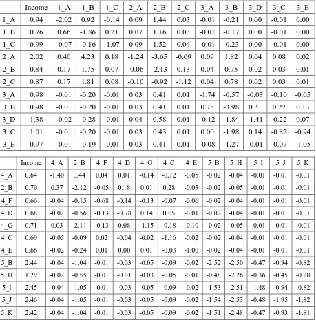
Elasticity estimates at the brand level are partly provided in Table I-8. An implication can be found between private labeled milk and brand milk products. Private labeled milk products (labeled as alphabet B in Table I-8) are substitutes for the other brand milk products in the same group while brand milk products are not substitutes for private labeled milk most of the case.

2) Variety Effects

computed at the original equilibrium. In other words, the index is computed with the mean values of market shares from post-introduction data. Although the differences between actual prices and virtual prices of each type of milk are large, the difference in the milk market index is small because the market share of organic milk is as small as 2.5% on average.

The variety effect is calculated with the formula given in section V which takes the curvatures of demand equations into account. The results imply that consumers in this data set obtain 838.8 dollars per month in total by having organic options in their choice sets and this is 8.2 percent of the milk expenditure. The benefit a representative consumer receives whenever he/she purchases a gallon of milk is 31 cents.

3) Price Effects

leading organic milk distributors, Horizon Organic, merged with a conventional dairy distributor, Dean Food, in 2004. Therefore, the coefficient of indicator valued one after 2004 might represent the competition between conventional and organic milk within the same manufacturers. Second, some of the negative price effects for the milk with higher fat contents can be explained by the demand shocks caused by consumers‟ health concerns on fat contents. Health related concerns on fat contents would cause positive demand shock in lower fat milk market and negative shock in higher fat milk market. The positive shock in lower fat market would lead to the price increase in the lower fat market and the negative shock would result in a lower price in the higher fat milk market.

Finally, the overall effect on consumer welfare of the organic milk introduction is calculated with the formula shown in section V. Since the variety effects and the price effects have opposite directions in this study, the estimates for compensating variation vary depending on the time and duration included in the computation.

VII. Conclusions

REFERENCES

Alviola IV, P. and Capps, Jr. O. (2010), “Household Demand Analysis of Organic and Conventional Fluid Milk in the United States Based on the 2004 Nielsen Homescan Panel”, Agribusiness, 26(3), 369-388.

Berry, S., J. Levinsohn, and A. Pakes (1995), “Automobile Prices in Market Equilibrium,” Econometrica, 63, 841-890.

Berry, S., J. Levinsohn, and A. Pakes (1998), “Differentiated Products Demand Systems from a Combination of Micro and Macro Data: The New Car Market,” NBER Working Paperno. 6481.

Carpentier, A. and Guyomard, H. (2001), “Unconditional Elasticities in Two-Stage Demand Systems: An Approximate Solution,” American Journal of Agricultural Economics, 83(1), 222-229.

Chavas, J.P., and Segerson, K., (1987), “Stochastic Specification and Estimation of Share Equation Systems”, Journal of Econometrics, 35, 337-358.

Deaton, A., Muellbauer, J. (1980), “Economics and Consumer Behavior,” Chaper 5 & 6, Cambridge University Press.

Dhar, T. and J. D. Foltz (2005), “Milk by Any Other Name … Consumer Benefits from Labeled Milk,” American Journal of Agricultural Economics, 87(1), 214-228.

Dimitri, C., and Greene, C., (2002), “Recent Growth Patterns in the U.S. Organic Foods Market,” Agricultural Information Bulletin, Economic Research Service/USDA.

Dimitri, C. and K. Venezia (2007), “Retail and Consumer Aspects of the Organic Milk Market,” A Report from Economic Research Service, USDA.

Garmon, J., S., Huang, C., L., and Lin, B., H. (2007), “Organic Demand: A Profile of Consumers in the Fresh Produce Market,” Choices, American Agricultural Economics Association, 22(2), 109-116.

Glaser, L. K., and Thompson, G. (2000), “The Demand for Organic and Conventional Milk,” Presented at the Western Agricultural Economics Association meeting, Vancouver, British Columbia.

Gorman, W.M. (1959), “Separable Utility and Aggregation,” Econometrica, 27(3), 469- 481. Harris, M. (2005): “Using Nielsen HomeScan Data and Complex Survey Design Techniques

Hausman J. (1981), “Exact Consumer‟s Surplus and Deadweight Loss,” The American Economic Review, 71(4), 662-676.

Hausman, J. (1996), “Valuation of New Goods under Perfect and Imperfect Competition,”in T. Bresnahan and R. Gordon, eds., The Economics of New Goods, Chicago: National Bureau of Economic Research.

Hausman, J., and Leonard, G. (2005), “The Competitive Analysis Using A Flexible Demand Specification,” Journal of Competition Law and Economics, 1(2), 279-301.

Hausman, J., Leonard, G., and Zona, J. D. (1994), “The Competitive Analysis with Differentiated Products,” Annales D’economie Et De Statistique, 34, 159-180.

Hausman, J., Leonard, G., and Zona, J. D. (2002), “The Competitive Effect of a New Product Introduction: A Case Study,” The Journal of Industrial Economics, 50(3), 237-263.

Hausman J., and Newey W. (1995), “Nonparametric Estimation of Exact Consumers Surplus and Deadweight Loss,” Econometrica, 63(6), 1445-1476.

Kao, C., Lee, L., and Pitt, M. (2001), “Simulated Maximum Likelihood Estimation of The Linear Expenditure System with Binding Non-negativity Constraints,” Annals of Economics and Finance, 2, 203-223.

Lohr, L. (2001), “Factors Affecting International Demand and Trade in Organic Food

Products.” In Changing Structure of Global Food Consumption and Trade, A. Regmi

(ed.). Agriculture and Trade Report No. WRS01-1. U.S. Department of Agriculture, Economic Research Service.

Lohr, L., and A. Semali (2000), “Retailer Decision Making in Organic Produce Marketing.”

In W.J. Florkowski, S.E. Prussia, and R.L. Shewfelt (eds.). Integrated View of Fruit and

Vegetable Quality. Technomic Pub. Co., Inc., Lancaster, PA. pp. 201-208.

Meyerhoeffer, C., Ranney, C, and Sahn, D. (2005), “Consistent Estimation of Censored Demand System Using Panel Data”, American Journal of Agricultural Economics, 87(3), 660-672.

Perali, F. and Chavas, J.P. (2000), “Estimation of Censored Demand Equations from Large Cross-Section Data,” Agricultural and Applied Economics Association, 82(4), 1022-1037. Strotz, R.H. (1957), “The Empirical Implications of a Utility Tree,” Econometrica, 25(2),

269-280.

Table I- 1 Distributions of Observed Household Attributes in the US

Income % Family Size %

Under $5000 0.82 Single

Member 25.35

$5,000 - $7,999 1.26 Two 37.99

$8,000 - $9,999 1.12 Three 15.03

$10,000 - $11,999 1.65 Four 13.17

$12,000 - $14,999 2.95 Five 5.55

$15,000 - $19,999 5.39 Six 1.93

$20,000 - $24,999 7.67 Seven 0.6

$25,000 - $29,999 6.74 Eight 0.26

$30,000 - $34,999 7.89 Nine+

Members 0.13

$35,000 - $39,999 6.92

$40,000 - $44,999 6.83

$45,000 - $49,999 6.39

$50,000 - $59,999 11.03

$60,000 - $69,999 8.86

$70,000 - $99,999 15.17

Table I-1 Continued

Age % Age of Child %

Under

25 Years 0.48 Under 6 only 3.78

25-29 2.9 6-12 only 6.32

30-34 6.33 13-17 only 8.11

35-39 8.95 Under 6 & 6-12 3.32

40-44 12.13 Under 6 & 13-17 0.55

45-49 13.73 6-12 & 13-17 4.3

50-54 13.18 Under 6 & 6-12 & 13-17 0.88

55-64 21.48 No Children

Under 18 72.74

65+ 20.83

Employment % Education %

Not Employed or

Part-time employed 37.78 Less than College 30.2

Table I- 2 Market Shares of Organic and Non-organic Milk by Observed Demographic Attributes at the National Level

Income Organic Conventional Family Size Organic Conventional

Under $5000 0.6 99.4 Single

Member 4.6 95.4

$5,000 -

$7,999 2.5 97.5 Two 2.9 97.1

$8,000 -

$9,999 4.6 95.4 Three 1.9 98.1

$10,000 -

$11,999 4.6 95.4 Four 2.3 97.7

$12,000 -

$14,999 0.6 99.4 Five 1.7 98.3

$15,000 -

$19,999 2.8 97.2 Six 0.6 99.4

$20,000 -

$24,999 2.6 97.4 Seven 0.1 99.9

$25,000 -

$29,999 1.7 98.3 Eight 0 100

$30,000 -

$34,999 0.9 99.1

Nine+

Members 0 100

$35,000 -

$39,999 3.1 96.9

$40,000 -

$44,999 3.3 96.7

$45,000 -

$49,999 2.3 97.7

$50,000 -

$59,999 3.6 96.4

$60,000 -

$69,999 1.7 98.3

$70,000 -

$99,999 2.6 97.4

100,000 &

Table I- 3 Continued

Age Organic Conventional Age of Child Organic Conventional

Under

25 Years 0.3 99.8 Under 6 only 2.7 97.3

25-29 3.6 96.4 6-12 only 1.9 98.1

30-34 1.9 98.1 13-17 only 1 99

35-39 3 97 Under 6 &

6-12 3.7 96.3

40-44 2.8 97.2 Under 6 &

13-17 15.2 84.8

45-49 1.9 98.1 6-12 & 13-17 2.2 97.8

50-54 3.5 96.5 Under 6 &

6-12 & 13-17 0.4 99.6

55-64 3 97 No Children

Under 18 2.9 97.1

65+ 2.6 97.4

Employment Organic Conventional Education Organic Conventional

Not Employed or Part-time

2.8 97.2 Less than

College 1.3 98.7

Full-time 2.7 97.3 College and

Table I- 4 Market Shares by Fat Contents and Organic Claim in the US

2002 2003 2004 2005

Non-Fat 23.89 24.03 24.51 27.63

1% Low Fat 16.92 17.05 18.17 20.06

2% Reduced 35.19 34.68 35.80 29.51

Whole Milk 21.41 20.78 18.28 19.00

Soy & Lactose Free 2.59 3.46 3.25 3.80

Non-Organic 98.38 97.75 97.81 97.53

Organic 1.62 2.25 2.19 2.47

Table I- 5 Market Share by Fat Contents and Organic Claim in RDU

2004 2005

Non-Fat 24.7 27.19

1% Low Fat 15.2 15.38

2% Reduced 30.62 28.38

Whole Milk 25.4 24.44

Soy & Lactose Free 4.08 4.61

Non-Organic 97.5 97.23

Table I- 6 Summary of Commodity Groups in RDU

Group Fat Organic Flavor Share Average Price

per Fluid Oz

Number of Brands

1 Non-Fat Nonorganic No flavor 24.59 0.028274 3

2 1% Low Fat Nonorganic No flavor 14.66 0.028336 3

3 2% Reduced Nonorganic No flavor 28.59 0.029892 5

4 Whole Milk Nonorganic No flavor 24.82 0.031272 7

5 Soy &

Lactose Free Nonorganic No flavor 1.67 0.048348 5

6 Non-Fat Organic No flavor 0.18 0.051564 3

7 1% Low Fat Organic No flavor 0.12 0.048173 2

8 2% Reduced Organic No flavor 0.14 0.052778 3

9 Whole Milk Organic No flavor 0.13 0.052442 4

10 Soy &

Lactose Free Organic No flavor 0.84 0.046248 3

11 Non-Fat Nonorganic Flavored 0.26 0.050497 2

12 1% Low Fat Nonorganic Flavored 0.3 0.037342 2

13 2% Reduced Nonorganic Flavored 0.6 0.054402 4

14 Whole Milk Nonorganic Flavored 1.21 0.047216 5

15 Soy &

Lactose Free Nonorganic Flavored 0.56 0.041551 4

16 Non-Fat Organic Flavored 0 n.a. 0

17 1% Low Fat Organic Flavored 0 n.a. 0

18 2% Reduced Organic Flavored 0 n.a. 0

19 Whole Milk Organic Flavored 0 n.a. 0

20 Soy &