Some Explicit Formulae of NAF and
its Left-to-Right Analogue
Dong-Guk Han1, Tetsuya Izu2, and Tsuyoshi Takagi1 1 FUTURE UNIVERSITY-HAKODATE,
116-2 Kamedanakano-cho, Hakodate, Hokkaido, 041-8655, Japan {christa,takagi}@fun.ac.jp
2 FUJITSU LABORATORIES Ltd.,
4-1-1, Kamikodanaka, Nakahara-ku, Kawasaki, 211-8588, Japan [email protected]
Abstract. Non-Adjacent Form (NAF) is a canonical form of signed bi-nary representation of integers. We present some explicit formulae of NAF and its left-to-right analogue (FAN) for randomly chosenn-bit in-tegers. Interestingly, we prove that the zero-run length appeared in FAN is asymptotically 16/7, which is longer than that of the standard NAF. We also apply the proposed formulae to the speed estimation of elliptic curve cryptosystems.
Keywords:signed binary representation, non-adjacent form, Hamming weight, zero-run length.
1
Introduction
In some exponentiation-based public-key cryptosystems including RSA and El-liptic Curve Cryptosystems (ECC), a binary representation of a given integer (which may be a secret in most cases) is commonly used as a standard tech-nique. While a non-signed representation of an integer is unique, we have some ways for representing the integer in signed form. For example, an integer 13 can be represented in signed form such as 10¯101, 100¯1¯1, or 10¯11¯1, where ¯1 denotes −1. Such signed binary representations are especially useful in ECC, since inver-sions of arbitrary points can be obtained with almost free operations over elliptic curves. Some properties of such signed binary representations are related to the cost of an exponentiation. Especially, the number of nonzero bits (the Hamming weight) is important since this value rules the number of multiplications in the exponentiation. Thus analyzing signed representations implies a cost evaluate of exponentiations.
The non-adjacent form (NAF) is a well-known signed binary representation [Rei60]. A NAF of a positive integerais an expressiona=Pni=0−1νi2iwhereνi∈ {−1,0,1}, νn−16= 0 and no two successive digits are nonzero, namelyνi·νi+1= 0 for i = 0,1, ..., n−2 [Rei60]. Each integer a has a unique NAF representation denoted byNaf(a). Moreover,Naf(a) can be efficiently computed by
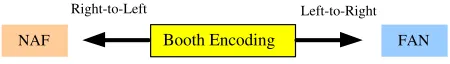
left-to-right analogue “FAN” 1. It is known that NAF and FAN can be generated by applying a sliding window method with width-2 to the Booth encoding [Boo51] in right-to-left and left-to-right, respectively [HKP+04,OSS+04]. Note that the Booth encoding was also introduced as the reversed binary representation by Knuth [Knu81, Exercise 4.1-27]. In this paper, the Booth encoding and FAN of an integeraare denoted byBooth(a) andFan(a), respectively.
Right-to-Left Left-to-Right
Booth Encoding FAN NAF
Fig. 1.A relation of the Booth encoding, NAF, and FAN.
NAF and FAN share some properties. Actually, they are generated by the similar manner as above, and the Hamming weights of NAF and FAN for the same integer are exactly same (Fact 1). In this paper, we prove an explicit formula derived from the Booth encoding (Theorem 1), which evaluates the average number of the Hamming weight of NAF and FAN representations as a first contribution. On the other hand, NAF and FAN have different properties. A fundamental observations is, while NAF does not have successive nonzero bits in the representation, FAN can have. Because of this difference, they have different significant length on average. We establish formulae for this value in Theorem 2. Moreover, we show the averaged length of zero runs in NAF and FAN in Theorem 3. In some implementations of ECC exponentiations, iterated elliptic curve doubling (wECDBL) is used for efficiency. With our analysis, a stricter evaluation of the averaged cost of exponentiations are possible. In fact, in ECC with 160-bit keys, FAN is about 15.97 multiplications (in a definition field) faster than NAF. Combined with a technique used in [SS01], FAN is about 317.47 multiplications faster than NAF.
An organization of this paper is as follows: section 2 defines some notations and the Booth encoding, NAF and FAN. In section 3, we prove some lemmas required for our theorems. Then, we establish an explicit evaluation formula for the Hamming weight in section 4. We also show evaluation formulae for the averaged significant length and the averaged zero runs (in NAF and FAN) in section 5, 6, respectively. Finally, in section 7, we apply our formulae to the cost evaluation of ECC exponentiations.
2
Preliminaries
2.1 Notations
For a givenn-bit integera=Pin=0−1ai2i withai∈ {0,1}, an
−1= 1, we use the following notations:
– Booth(a),Naf(a), andFan(a) denote the Booth encoding, NAF, and FAN
representation of the integerarespectively. • Booth(a) :=Pn
i=0βi2i withβi∈ {−1,0,1}, • Naf(a) :=Pn
i=0νi2i withνi ∈ {−1,0,1}, • Fan(a) =Pn
i=0φi2i withφi∈ {−1,0,1}.
– B(n) :={Booth(a)|0≤a≤2n−1}.
• Case I B(n) :={Booth(a) withβn= 0| 0≤a≤2n−1}.
• Case II B(n) :={Booth(a) with (βn, βn−1) = (1,¯1)|0≤a≤2n−1}.
• Case III B(n) :={Booth(a) with (βn, βn−1) = (1,0)|0≤a≤2n−1}. – N(n) :={Naf(a)|0≤a≤2n−1}.
– F(n) :={Fan(a)|0≤a≤2n−1}. – κn= 2 ifnis odd and κn = 1 ifnis even.
– εn is the negligible function in n, namely for every constant c ≥ 0 there exists an integernc such that|εn| ≤1/nc for alln≥nc.
2.2 Booth Encoding, NAF and FAN
The Booth encoding [Boo51] of an integer is defined as follows:
Definition 1 (Booth Encoding [OSS+04]).Then-bit Booth encoding is an
n-bit signed binary representation that satisfies the following two conditions: 1. Signs of adjacent nonzero bits (without considering zero bits) are opposite. 2. The most nonzero bit and the least nonzero bit are 1 and ¯1, respectively,
unless all bits are zero.
In [OSS+04], they showed a simple conversion method from ann-bit binary string to (n+ 1)-bit Booth encoding. Given an integera, the Booth encoding of ais obtained by
Booth(a) = 2a a,
where stands for a bitwise subtraction.
The non-adjacent form (NAF) also represents an integer in signed form. Since there is no successive nonzero bits in the representation, NAF is a standard tech-nique for computing exponentiations [IEEE]. According to [HKP+04,OSS+04], NAF can be interpreted as a combination of the Booth encoding and a right-to-left sliding window method with width-2. For example, for an integer 13, we haveBooth(13) = 10¯11¯1. Then we divideBooth(13) (as a string) into width-2
windows from right to left: 01, 0¯1, 1¯1 (the leftmost 0 was padded), and convert 1¯1 to 01 and ¯11 to 0¯1, if exist. Thus we haveNaf(13) = 10¯101.
FAN was introduced as a left-to-right analogue of NAF [JY00]. In fact, FAN can be also interpreted as a combination of the Booth encoding and a left-to-right sliding window method with width-2. For example, again, we divide the Booth encoding Booth(13) = 10¯11¯1 into width-2 windows from left to right:
10, ¯11, ¯10 (the rightmost 0 was padded). Then, similarly to NAF, convert 1¯1 to 01 and ¯11 to 0¯1, if exist. Thus we haveFan(13) = 100¯1¯1. Note that FAN can
have successive nonzero bits unlike NAF.
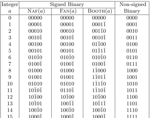
Integer Signed Binary Non-signed
a Naf(a) Fan(a) Booth(a) Binary
0 00000 00000 00000 0000
1 00001 00001 0001¯1 0001 2 00010 00010 001¯10 0010 3 0010¯1 0010¯1 0010¯1 0011 4 00100 00100 01¯100 0100 5 00101 00101 01¯11¯1 0101 6 010¯10 010¯10 010¯10 0110 7 0100¯1 0100¯1 0100¯1 0111 8 01000 01000 1¯1000 1000 9 01001 01001 1¯101¯1 1001 10 01010 01010 1¯11¯10 1010 11 10¯10¯1 0110¯1 1¯110¯1 1011 12 10¯100 10¯100 10¯100 1100 13 10¯101 100¯1¯1 10¯11¯1 1101 14 100¯10 100¯10 100¯10 1110 15 1000¯1 1000¯1 1000¯1 1111
Table 1.NAF, FAN, Booth encoding representations of some integers
3
Lemmas
In this section, we prepare some lemmas required to prove our theorems.
3.1 Some Properties of Booth Encoding
Property 1. Due to the definition of Booth encoding, the number of Hamming weight ofBooth(a) is always even, if the original integerais positive.
Let h1¯1ik be a pattern of nonzero bits in Booth encoding such that k
z}|{
1,¯1, . . . , 2
z}|{
1,¯1, 1
z}|{
1,¯1 (k-times) without considering zero bits between 1 and ¯1. Let #[h1¯1ik] be the total number of strings with h1¯1ik pattern. For exam-ple, in B(3)\ {0}, all elements except 1¯11¯1 have the same patternh1¯1i2. Thus #[h1¯1i2] = 6 and #[h1¯1i4] = 1.
Lemma 1 (Pattern Lemma). B(n)contains all possible representations with
h1¯1ik pattern for 0≤k≤ dn/2e.
Proof. For 1≤k≤ dn/2e,
#[h1¯1i0] = n+ 1 0
!
, #[h1¯1i1] = n+ 1 2
!
, . . .
#[h1¯1ik] = n+ 1 2k
!
, . . . #[h1¯1idn/2e] = n+ 1 2dn/2e
!
ThusPdkn/=02e#[h1¯1ik] =Pdn/2e
k=0 n+1
2k
= 2n. This implies that there are 2n different representations withh1¯1ikpattern. As the total number of integers with n-bit is 2nand Property 1, the assertion is proved. ut
Lemma 2 (Classification Lemma). B(n) can be divided into the following three cases;
– Case I B(n)with#[Case I B(n)]=2n−1,
– Case II B(n)with#[Case II B(n)] = 2n−2,
– Case III B(n)with #[Case III B(n)] = 2n−2.
Proof. From Property 1 and Lemma 1,
#[Case I B(n)] =
bn 2c
X
k=0
n
2k
!
= 2n−1,
#[Case II B(n)] =
bn−1 2 c
X
k=0
n−1 2k
!
= 2n−2,
#[Case III B(n)] =
Pbn−1
2 c
k=0 n−1 2k+1
, (ifnis even) Pbn−1
2 c−1
k=0
n−1 2k+1
, (otherwise)
= 2n−2.
u t
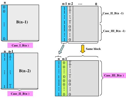
Lemma 3 (Extension Lemma). B(n) can be constructed fromB(n−1) ac-cording to the following rules;
– Case I B(n) ={(βn= 0)k(βn−1, . . . , β0)|(βn−1, . . . , β0)∈ B(n−1)},
– Case II B(n)=(βn, βn−1)=(1,¯1)k(βn−2, . . . , β0) |(βn−2, . . . , β0)∈ B(n−2) ,
– Case III B(n)=(βn, βn−1)=(1,0)k(βn−2,. . . ,β0)|(1, βn−2,. . . ,β0)∈{Case II B(n−1) ∪Case III B(n−1)} .
Here,xy denotes concatenation between two bit stringsxandy.
Proof. From Property 1 and Lemma 1, 2, we can see that the assertion is true.
In the third case, in order to construct Case III B(n) the most bit 1 of the strings sampled from{Case II B(n−1)∪Case III B(n−1)}is changed to βn−1= 0 andβn= 1 is concatenated. Refer to Fig. 2.
Lemma 4 (Case II-Classification Lemma).
#Case II B(n)with#(the most consecutive nonzero bits) =even= 2n−1+κn
3 ,
#Case II B(n)with #(the most consecutive nonzero bits) =odd= 2n−2−κn
3 ,
whereκn= 2 ifn is odd andκn= 1 ifnis even. Especially,
#Case II B(n)with#(the most consecutive nonzero bits) = 2= 2n−3.
1 1 1 1 1 1 1 1 1 0 0 0
n-1 n-2 … 0
Case_II_B(n -1) Case_III_B(n -1) . .. . .. ... . .. 1 1 1 1 1 1 . .. . .. 0 0. .. 0 0 0. .. 0 Case_III_B(n ) 1 1 1 0 0 0 . .. . .. Same block B(n-1) 0 0 . .. 0 Case_I_B(n ) B(n-2) 1 1 1 . .. 1 1 1 ... Case_II_B(n ) n-1 n n n-1 n
Fig. 2.ConstructB(n) fromB(n−1)
3.2 Relations among Booth, NAF, and FAN
Lemma 5 (Adjacent Lemma). The string with odd(>1)number of consec-utive nonzero bits in Booth representations is converted into a sting with 11or
¯1¯1in FAN representation.
Booth
z }| {
. . .0 1¯11¯1· · ·1¯11 | {z }
#odd
0. . .⇒
F AN
z }| {
. . .0 0101· · ·011 | {z }0. . .,
Booth
z }| {
. . .0 ¯11¯11· · ·¯11¯1 | {z }
#odd
0. . .⇒
F AN
z }| {
. . .0 0¯10¯1· · ·0¯1¯1 | {z }0. . .
However, the even number of consecutive nonzero bits in Booth representations is not converted into 11or¯1¯1.
Lemma 6 (Length Lemma).For a given n-bit integer a, i.e. an−1= 1, L[Booth(a) with (bn, bn−1) = (1,0)]
=L[Naf(a)] =L[Fan(a)],
L[Booth(a) with #(the most consecutive nonzero bits) =even]
=L[Naf(a)] + 1 =L[Fan(a)] + 1,
L[Booth(a) with #(the most consecutive nonzero bits) =odd(>1)]
=L[Naf(a)] =L[Fan(a)] + 1.
From the results of Lemma 6, we prove the followingNAF Carry Formulaof NAF.
Lemma 7 (NAF Carry Formula). Assume that NAF is converted from in-tegers ofn bits. The carry at(n+ 1)-th bit of NAF occurs with probability
Cn= 1 3−
κn 3
1 2
n
, (1)
whereκn= 2 for oddnandκn= 1 for evenn.
Proof. Consider B(n). From Lemma 6, the elements of Case III B(n) and
Case II B(n) with #(the most consecutive nonzero bits)= odd (>1) are con-verted into NAF with a carry at (n+ 1)-bit. From Lemma 2 and 4, the total number of integers with a carry at (n+ 1)-bit is equal to
2n−2+2
n−2−κn
3 =
2n−κn
3 ,
whereκn= 2 for oddnandκn= 1 for evenn. Thus the carry probabilityCn is 1
3− κn
3 1 2
n .
4
Hamming Weight of NAF and FAN
This section shows an explicit evaluation formula for the Hamming weight of NAF and FAN. The following fact is fundamental for our discussion.
Fact 1 (Theorem 12. [JY00,HKP+04]) The Hamming weight of NAF is exactly equal to that of FAN for each integer.
LetH(a) be the Hamming weight ofNaf(a). LetH(n) be the average
Ham-ming of NAF forn-bit integers, which is defined by
H(n) =
P2n
−1 k=0 H(k)
2n . (2)
For example, H(2) = 1,H(3) = 118,H(4) = 74,H(5) = 6732. Then, we have the following theorem.
Theorem 1. Let nbe any integer larger than1. The average Hamming weight of the NAF and FAN ofn-bit integers is
H(n) = 1 3n+
4 9 −
κn+ 3 9
1 2
n
, (3)
whereκn= 2 for oddnandκn= 1 for evenn.
1. First find the average Hamming weight of B(n). (Refer to Lemma 8) 2. Next find the average number of two consecutive nonzero bits appeared in
B(n). (Refer to Lemma 9)
3. The wanted average Hamming weight of NAF is
[Result of Step1]−[Result of Step2].
u t
Lemma 8. The average Hamming weight of Booth representations in B(n)is
HBooth(n) = 1 2n+
1
2. (4)
Proof. From Lemma 1, the total number of Hamming weight of Booth is
2· n+ 1 2
!
+ 4· n+ 1 4
!
+. . .+ 2k· n+ 1 2k
!
+. . .+ 2dn/2e · n+ 1 dn/2e !
= (n+ 1)2n−1.
ThereforeHBooth(n) = (n+1)2
n−1
2n =
n 2 +
1 2.ut
We investigate the average number of two consecutive nonzero bits appeared in the representation of BoothB(n). Indeed we prove the following theorem.
Lemma 9. Assume that Booth is converted from integers ofnbits. The average number of two consecutive nonzero bits appeared in the representation of Booth is
An= 1 6n+
1 18+
κn+ 3 18
1 2
n−1
, (5)
whereκn= 2 for oddnandκn= 1 for evenn.
Proof. LetBn be the total number of two consecutive nonzero bits appeared in B(n). For example, we knowB2= 2,B3= 5, B4= 12, andB5= 29.
Now we prove that the following relationship holds.
Bn= 2Bn−1+
2n−1−κn
3 , (6)
where κn = 2 if oddn and κn = 1 if even n. From Lemma 2, there are three cases: (1) the most bit is 0, (2) the most two bits are 1¯1, and (3) the most two bits are 10.
– In the case of (1), the number of two consecutive nonzero bits isBn−1.
– In the case of (3), we know that it is related with the Case II and III of B(n−1). The number of two consecutive nonzero in B(n) derived from Case III B(n−1) is exactly equal to that ofCase III B(n−1). However, there are some changes if the target part of B(n) which is derived from Case II B(n−1). That is if the number of the most consecutive nonzero bits is even in the Case II B(n−1) then the number of two consecutive nonzero bits is decreased by one inB(n). (Refer to Lemma 2 and 3.) From Lemma 4, #[Case II B(n−1) with #(the most consecutive nonzero bits) = even] = 2n−2+κn
3 , where κn = 2 if odd n and κn = 1 if even n. Therefore it is equal toBn−1−Bn−2− 2
n−2
+κn
3
.
Summing up those three values we obtain equation (6). FromAn =Bn/2n and equation (6), we obtain
An=An−1+ 1 3
1
2 −κn 1 2
n
. (7)
Then we know
An=A2+ 1 3
n
X
i=3
1
2 −κn 1 2
i
= 1 6n+
1 18+
κn+ 3 18
1 2
n−1 ,
whereκn= 2 for oddnandκn = 1 for evenn.ut
5
Bit Length of NAF and FAN
This section shows an evaluation formulae for the averaged siginificant length of NAF and FAN, which are summarizes in the following theorem.
Theorem 2. Let nbe any integer larger than 1. The average significant length of NAF and FAN is
LN(n) =n−1 3+
−1 2n+
1 3κn
1 2
n
, (8)
LF(n) =n−1
2, (9)
whereκn= 2 for oddnandκn= 1 for evenn.
2nLF(n) = (n+ 1)2n−2+ n−2
X
i=1
(i+ 2)(2i+ 2i−1) + 2·1 + 1·1 =n2n−2n−1,
LF(n) =n−1 2.
Next we estimate the average significant length of NAF denoted asLN(n). From Lemma 6, the following equation holds.
2nLN(n) = 2nLF(n)
+ n
X
i=4
#[Case II B(i)with#(the most consecutive nonzero bits) =odd].
From Lemma 4, n
X
i=4
#[Case II B(i)with#(the most consecutive nonzero bits) =odd]
=
(Pn−3
2
i=1 2
2i−1
3 +
Pn−3 2
i=1 2
2i+1−2
3 =
2n−1
3 −
n 2 +
1
6 (if nis odd)
Pn−2 2
i=1 2
2i
−1
3 +
Pn−4 2
i=1 2
2i+1
−2
3 =
2n−1
3 −
n 2 +
1
3 (if nis even) = 2
n−1
3 −
n 2 +
1 3κn,
whereκn= 2 ifnis odd and κn = 1 ifnis even. Thus
2nLN(n) = 2n
n−1 2
+2 n−1
3 −
n 2 +
1 3κn,
LN(n) =n−1 3+
−1 2n+
1 3κn 1 2 n .
6
Zero Run Length of NAF and FAN
In this section, we investigate the averaged length of zero run regarding to NAF and FAN. For example, the average length of zero run for 10¯10¯101 is 1. The corresponding FAN is 1100¯1¯1 and its average length of zero run is 2. In general FAN has a longer zero run on average. Indeed we prove the following theorem.
Theorem 3. The average zero run of NAF and FAN converted from n bits integers is equal to
LN(n)− H(n) H(n)−1
2 =
2 3n−
7 9+εn 1
3n− 1 18+εn
= 2 +O(n−1), LF(n)− H(n)
H(n)−1 2−
En
2n
= 2 3n−
17 18+εn 7
24n− 5 72+εn
=16 7 +O(n
respectively. Here we define
En= 1 24n2
n−6 + 2κn
9 + (
1 72)·2
n,
whereκn= 2ifnis odd andκn = 1ifnis even, andεnis the negligible function inn.
Proof. At first we estimate the average zero run of NAF. The total number of zero appeared in NAF converted from n bits integers is LN(n)2n − H(n)2n. Because there is no consecutive nonzero bits, the number of zero runs can be estimated by Hamming weight, namely there are H(n)2n−2n−1 different zero runs, where 2n−1 is the number of NAF whose least bit is nonzero. Therefore, the average length of zero run for NAF is evaluated as follows:
LN(n)2n− H(n)2n H(n)2n−2n−1 =
LN(n)− H(n) H(n)−1
2 =
2 3n−
7 9+εn 1
3n− 1 18+εn
= 2 +O(n−1),
whereεnis the negligible function inn. Next we estimate the average number of zero run for FAN. The number of two consecutive nonzero bits 11 and ¯11 should be excluded from the number of different consecutive zeroes appeared in the denominator above. In the following we estimate the number these exceptional consecutive bits. LetEnbe the number of 11 and ¯11 appeared in FAN converted fromnbits integers. We know E4= 2, E5= 6,andE6= 16.
We use the three cases appeared in Lemma 2: (1) the most bit is 0, (2) the most two bits are 1¯1, and (3) the most two bits are 10. The estimation is similar to Lemma 9.
– In the case of (1), the number isEn−1.
– In the case of (2), from Lemma 3 the target part ofB(n) is (1¯1)B(n−2). From Lemma 5 we can see that only the strings such that (βn−2, βn−3) = (1,0) inB(n−2) generate new 11 inB(n). Thus the number isEn−2+ 2n−4.
– In the case of (3), the number of two consecutive nonzero bits inB(n) de-rived fromCase III B(n−1) is exactly equal to that ofCase III B(n−1). However, there are some changes if the target part ofB(n) which is derived fromCase II B(n−1) because #(the most consecutive nonzero bits)≥2. We considerCase II B(n−1). From Lemma 5, we can derive the following results;
• If #(the most consecutive nonzero bits) = 2 then there is no change of the number of two consecutive nonzero bits.
• If #(the most consecutive nonzero bits) = even(> 2) then new 11 is generated after conversion to FAN.
Thus the number is
En−1−En−2
+ #Case II B(n−1)with#(the most consecutive nonzero bits) =even(>2) −#Case II B(n−1)with#(the most consecutive nonzero bits) =odd
=En−1−En−2+
4−κn2n−4 3κn
,
whereκn= 2 ifnis odd andκn= 1 ifnis even. (Refer to Lemma 4.)
Therefore we have the following relationship:
En= 2En−1+
κn2n−3+ 4
3κn ,
whereκn= 2 ifnis odd and κn = 1 ifnis even. Thus we obtain
En= 1 24n2
n−6 + 2κn
9 + (
1 72)·2
n,
whereκn= 2 ifnis odd and κn = 1 ifnis even.
Therefore, the average length of zero run for FAN is evaluated as follows:
LF(n)2n− H(n)2n H(n)2n−2n−1−En =
2 3n−
17 18+εn 7
24n− 5 72+εn
= 16 7 +O(n
−1).
7
Application to ECC
In this section we estimate the efficiency of scalar multiplication used for ECC with NAF or FAN. We assume that the scalar is a randomly chosenn-bit integer. LetECDBLandECADDbe the efficiency of computing elliptic doubling and
addition, respectively. The average number of multiplication for computing scalar multiplications using NAF or FAN is estimated by
(LN(n)−1)ECDBL+ (H(n)−1)ECADD (10)
(LF(n)−1)ECDBL+ (H(n)−1)ECADD. (11)
From Theorem 2, the difference of average efficiency is equal to
1
6 +
−1 2n+
1 3κn
1 2
n
ECDBL, (12)
whereκn= 2 for oddnandκn = 1 for evenn.
multiplications (4M+6S) [CMO98]. For example, ECC with 160 bits (n= 160) using FAN is about 1.47 multiplications faster on average than that using NAF. If ECDBL is repeatedly computed w times, we have an efficient variation,
calledwECDBL that can be computed with 4wM+ (4w+ 2)S [ITT+99].
The difference of average efficiency from Theorem 3 is equal to
n w1
∗(7.2∗w1+ 1.6)− n w2
∗(7.2∗w2+ 1.6), (13)
where w1 and w2 denote the expected number of wfor NAF and FAN respec-tively, and actuallyw1= 1.987 andw2= 2.269 forn= 160. Therefore the result equation (14) is 15.97. This implies that FAN is about 15.97 multiplications faster than NAF.
If we consider Sakai-Sakurai method [SS01] of multidoubling for Weierstrass elliptic curves in terms of affine coordinates that can be computed with (4w+ 1)M + (4w+ 1)S+I. Whenn= 160 the difference of average efficiency is
n w1
∗(7.2∗w1+ 31.8)− n w2
∗(7.2∗w2+ 31.8) = 317.47,
i.e. FAN is about 317.47 multiplications faster. Here,w1= 1.987 andw2= 2.269 forn= 160.
Acknowledgements
Dong-Guk Han was supported by the Korea Research Foundation Grant. (KRF-2005-214-C00016)
References
[Boo51] A. Booth, “A signed binary multiplication technique”, Journ. Mech. and Ap-plied Math., 4(2), pp.236-240, 1951.
[CMO98] H. Cohen, A. Miyaji, and T. Ono, “Efficient elliptic curve exponentiation using mixed coordinates,” Asiacrypt’98, LNCS 1514, pp.51-65, Springer-Verlag, 1998.
[HKP+04] C. Heuberger, R. Katti, H. Prodinger, and X. Ruan, “The alternat-ing greedy expansion and applications to left-to-right algorithms in cryptog-raphy”, To appear in Theor. Comput. Sci. A. Preprint version is available at http://www.opt.math.tu-graz.ac.at/ cheub/publications/alg1.pdf
[IEEE] IEEE 1363-2000, IEEE Standard Specifications for Public-Key Cryptography, 2000.
[ITT+99] K. Itoh, M. Takenaka, N. Torii, S. Temma, and Y. Kurihara, “Fast Im-plementation of Public-Key Cryptography ona DSP TMS320C6201,”CHES’99, LNCS 1717, pp.61-72, Springer-Verlag, 1999.
[JY02] M. Joye, and S.-M. Yen, “New minimal modified radix-r representation with ap-plications to smart-cards”, Proc. of PKC 2002, LNCS 2274, pp. 375-383, Springer-Verlag, 2002.
[Knu81] D.E. Knuth, ”The Art of Computer Programming, vol. 2, Seminumerical Al-gorithms, 2nd ed., Addison-Wesley, Reading, Mass, 1981.
[OSS+04] K. Okeya, K. Schmidt-Samoa, C. Spahn, and T. Takagi, “Signed Binary Representations Revisited”, IACR Cryptology ePrint Archive, 2004. Available at http://eprint.iacr.org/2004/195
[Rei60] G.W. Reitwiesner, Binary arithmetic, Advances in Computers, vol.1, pp.231-308, 1960.