Half Logistic Software Reliability Growth Model

International

 

Journal

 

of

 

Advanced

 

Research

 

in

 

Computer

 

Science

 

RESEARCH PAPER 

Available Online at www.ijarcs.info 

Half Logistic Software Reliability Growth Model

Dr.R.Satya Prasad *

Dept. of Computer Science Engineering Acharya Nagarjuna University

[email protected]

Dr.R.R.L. Kantam

Department of Statistics Acharya Nagarjuna University

[email protected]

Abstract: A software reliability growth model based on non- homogeneous Poisson process (NHPP) is derived with its mean value

function satisfying conditions similar to those of Goel and Okumoto (1979) and Musa and Okumoto (1984). The model turned out to be the (folded) half logistic distribution of Balakrishnan (1985). Reliability performance measures of the model are presented. Its parameters are estimated by maximum likelihood and approximate maximum likelihood methods. Asymptotic dispersion ma-trix, interval estimation also are derived. The results are illustrated with software failure data. The performance of the proposed model is evaluated in relation that of Goel and Okumoto (1979)

Keyword: Count process, mean value function, intensity function, software reliability, maximum likelihood estimation.

I. INTRODUCTION

Software reliability is the probability of failure free opera-tion of a computer program in a specified environment for a specified time. A failure is a departure of a program opera-tion from program requirements. A software reliability model provides a general form in terms of a random process describing failures for characterizing software reliability or a related quantity as a function of experienced failures over time.

In this backdrop Musa and Okumoto (1984) suggested a model for software reliability measurement and named it as logarithmic Poisson execution time model (LPETM). Motivated by their approach we develop a new software reliability model in this paper and present its performance in measuring software reliability. The development of our model, the reliability measurement characteristics and esti-mation procedures associated with it are given in Sections 2, 3, 4 respectively. Illustration of the results and the evalua-tion of the proposed model with a live data are presented in section 5.

II. THE PROPOSED MODEL

Let

⎡

⎣

N t , t 0 , m t ,

( )

≥

⎤

⎦

( ) ( )

λ

t

be the counting process, mean value function and intensity function of a software failure phenomenon. LPETM was derived with the following assumptions:

Assumption (i): There is no failure observed at time t

= 0. That is, N (0) =0 with probability one.

Assumption (ii): The failure intensity

λ

( )

t

will

de-crease exponentially with the expected number of failures experienced up to time‘t’ so that the relation between m (t) and

λ

( )

t

is

( )

( )

0

.

m t

t

e

θ

λ

=

λ

−

(1)

Where

λ

₀ and

θ

are the initial failure intensity and the rate of reduction in the normalized failure intensity per failure respectively.

Assumption (iii): For a small interval

Δ

t

the

prob-abilities of one, more than one failure during

[

t,t+ t

Δ

]

are

λ

( )

t

.

Δ + Δ

t

0( )

t

And

0( )

Δ

t

, respectively, where

0( )

0

t

t

Δ

→

Δ

as

Δ →

t

0

. Note that the probability of no

failure during

[

t,t+ t

Δ

]

is given by

1

−

λ

( )

t

Δ + Δ

t

0(

t

)

. Using assumptions (i) and (ii) the mean value function and intensity function are derived to be

0

1

( )

log(

1)

m t

λ θ

t

θ

=

+

(2)

0

0

( )

(

1

t

t

)

λ

λ

λ θ

=

+

(3)

It may be noted that as . Hence this model is also called ‘infinite failures’ model. Using as-sumptions (i) and (iii) the probability distribution of the sto-chastic process N(t) is given by

( )

m t

→ ∞

t

→ ∞

[

( )

] [

( )

]

.

( )

!

y m t

m t

P N t

y

e

y

−

=

=

(4)

0,

0

Here ‘a’ represents the expected number of software failures eventually detected. If

λ

( )

t

is the corresponding intensity function, the basic assumption of LPETM says that

( )

t

λ

is a decreasing function of as a result of repair action following early failures. We model this assumption as a relation between and

( )

m t

( )

m t

λ

( )

t

so that one can be ex-pressed in terms of the other. Our proposed relation is

2 2

Where ‘b’ is a positive constant, serving the purpose of constant of proportional fall in

λ

( )

t

. This relation indicates

a decreasing trend for

λ

( )

t

with increase in - a char-acteristic similar to that of LPETM which requires exponen-tial decrease of

( )

m t

( )

t

λ

with increase in , whereas our proposed model requires a quadratic decrease of

( )

m t

( )

t

λ

with . According to our proposition we get the follow-ing differential equation

( )

Whose solution is

(

)

We propose an NHPP with its mean value function given in equation (5). Its intensity function is

(

)

2

Our proposed model is derived on lines of Goel and Okumoto (1979) specifying a relation between m(t) and λ(t) as motivated from LPETM .Our model turns out to be the probability model of half logistic distribution of Balakrish-nan (1985). This model is paid a considerable attention as a reliability model recently by many authors and some of those published works are Kantam et al.,(1994), Kantam and

Dharmarao (1994), Kantam and Rosaiah (1998), Kantam et al.,(2000), Kantam and Srinivasarao (2004) and the

refer-ences therein. In short, we abbreviate this model as HLSRGM.

III. RELIABILITY PERFORMENCE MEASURES

Using the mean value function m(t) for HLSRGM, the probability distribution of the counting process N(t) is given by dom number of failures experienced by time ‘t’. Suppose that y

( )

m t

e failures have been observed during

[ ]

0,

t

e . Then the con-ditional distribution of N(t) given for is

the distribution of number of failures during

( )

_{e e} The probability that exceeds a real number ‘x’ given that the total time up to the (K-1)

k

Equation (9) is called the software reliability. If we take the negative of derivative of Equation (9) with respect to x, we get the conditional density as

[ ( ) ( )]

The hazard rate is given by the ratio of density to reli-ability which becomes

1

( k/ k ) ( )

h X S ₋ =

λ

s+x

(11)

In equations (9), (10) and (11) the expressions for m(t) and λ(t) are given by the respective quantities of HLSRGM.

IV. ESTIMATION BASED ON INTER FAILURE TIMES

We may recall that the mean value function and inten-sity function of HLSRGM are given by

(

)

The constants ‘a’, ’b’ which appear in the mean value function and hence in NHPP, in intensity function (error detection rate) and various other expressions are called pa-rameters of the model. In order to have an assessment of the software reliability ‘a’,’ b’ are to be known or they are to be estimated from a software failure data. Suppose we have ‘n’ time instants at which the first, second, third..., nth _{failures of}

software are experienced. In other words if is the total time to the k

k

S

th _{failure, is an observation of random}

vari-able and ‘n’ such failures are successively recorded, the k

s

k

joint probability of such failure time realizations

The function given in equation (14) is called the likeli-hood function of the given failure data. Values of ‘a’, ‘ b’ that would maximize L are called maximum likelihood es-timators (MLEs) and the method is called maximum likeli-hood (ML) method of estimation. Accordingly ‘a’, ‘b’ would be solutions of the equations

log

log

Substituting the expressions for m(t), λ(t) given by eq-uations (12) and (13) in equation (14), taking logarithms, differentiating with respect to ‘a’, ‘b’ and equating to zero, after some joint simplification we get

(

)

MLE of ‘b’ is an iterative solution of equation (16) which when substituted in equation (4.4) gives MLE of ‘a’. In order to get the asymptotic variances and co-variance of the MLEs of ‘a’, ‘b’ we need the elements of the informa-tion matrix which can be obtained through the following second order partial derivatives.

2

Expected values of negatives of the above three deriva-tives would be the following information matrix

2 2

Inverse of the above matrix is the asymptotic variance covariance matrix of the MLEs of ‘a’,‘ b’. Generally the

above partial derivatives evaluated at the MLEs of ‘a’, ‘b’ are used to get consistent estimator of the asymptotic vari-ance covarivari-ance matrix.

In order to overcome the numerical iterative way of solving the log likelihood equations and to get analytical estimators rather than iterative, some approximations in es-timating the equations can be adopted from Kantam and Dharmarao (1994), Kantam and Sriram (2001) and the ref-erences therein. We use two such approximations here to get modified MLEs of ‘a’ and ‘b’.Equation (4.5) can be written as

Let us approximate the following expressions in the L.H.S of equation (20) by linear functions in the neighbor-hoods of the corresponding variables.

.

(21) and (22) are to be suitably found. With such values, equations (21) and (22) when used in equation (4.9) would give an approximate MLE for ‘b’ as

1

We suggest two methods to get the slopes and inter-cepts in the R.H.S of equations

(21) and (22)

Given a natural number ‘n’ we can get the values of

i

u and u

′

_i

′′

by inverting the above equations through the function F(z). If G (.), H (.) are the symbols for the L.H.S of equations (21) and (22) we get

( )

n

( )

n based on only a specified natural number ‘n’ and can be computed free from any data. Given the data observations and sample size using these values along with the sample data in equation (4.12) we get an approximate MLE of ‘b’. Equation (4.4) gives approximate MLE of ‘a’.

Method II.

In this method we consider the Taylor series expansion up to the first derivative of the functions G (.), H (.) around and respectively where

u

is the solution of the following equations

, (

1, 2,.... )

Accordingly the expressions for the slopes and inter-cepts of equation (4.10) and (4.11) are given by

( )

( )

As mentioned in method I, here also the slopes and in-tercepts can be calculated free from magnitudes of data ob-servations. These values when used in equation (4.9) would give another approximate MLE of ‘b’ and subsequently an-other approximate MLE of the parameter ‘a’ from equation (4.4). Thus given software failure data in the form of inter failure times of a finite number of failures in terms of

X

_kor

k

S

we can get estimates of the parameters ‘a’, ‘b’, of HLSRGM by exact ML method as iterative solution of equation (4.5) and an approximate MLE by two methods of approximation as described above. In the case of approxima-tions, the basic principle is, some expressions of the estimat-ing equations are approximated by linear functions. The larger the size of the sample the closer the approximation. Hence the exactness of the approximation becomes finer for large values of ‘n’. Therefore, approximate MLEs and exact MLEs differ little, when the number of experienced software failures is large. As supported by Bhattacharya (1985), we can consider approximated expressions of log L for the ele-ments of the information matrix in order to get the

asymp-totic variances and covariance of the estimators of a, b. Hence

Estimated variances and covariance of are ob-tained from the elements of the inverse of the matrix evalu-ated at

a

.

which can be used to get the estimated asymptotic vari-ance of estimate of any reliability characteristic like mean value function, intensity function, reliability function etc., In all these cases a software reliability characteristic is a para-metric function say g(a, b). Estimated asymptotic variance of estimate of g(a, b) is given by

With the help of asymptotic optimum properties of MLEs, we can get the

(

1

−

α

)

z

−

%

equitable confidence in-tervals for ‘a’,’b’ or any parametric function of ‘a’,’b’ using the elements of inverse of the matrix (27) or the R.H.S of equation (28) evaluated at

a b

ˆ,

ˆ

.That is, dard normal distribution.

)

chi-square distribution with 2 degrees of freedom,

og

( )

( )

( )

of a chi-square distribution with 2 degrees of freedom. The procedure of interval estimation described above can be adopted by using the exact MLEs of ‘a’, ‘b’ and the corre-sponding estimated variances, covariance of the MLEs with the help of equations (15) through (19).

V. ILLUSTRATION AND EVALUATION OF THE MODEL

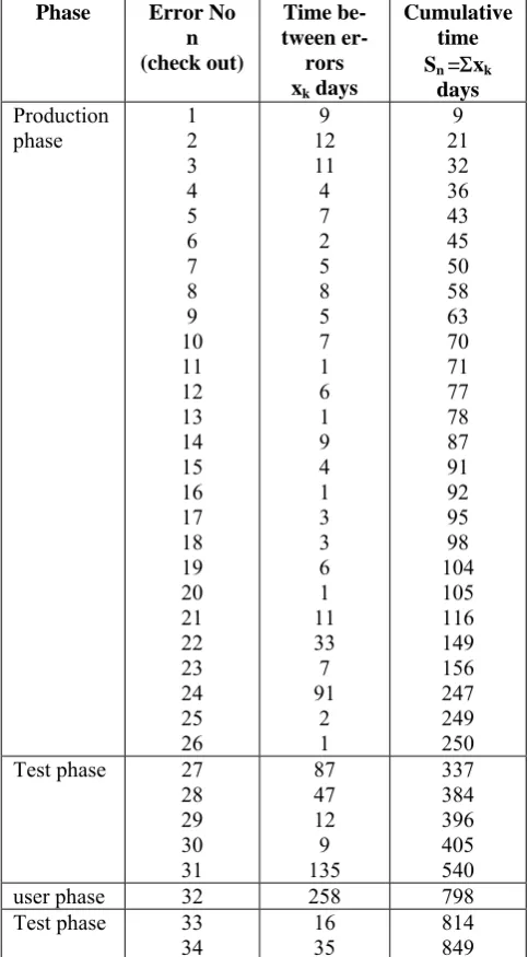
We apply the results to the software failure data of Na-vel Tactical Data system (NTDS) borrowed from Jelinski and Moranda (1972), given in the following table.

Table I: Software failure data

Phase Error No

We confirm the suitability of our model to the data by a test of goodness of fit known as Q-Q plot. We have taken the first 26 observations for the Q-Q plot. The correlation

coefficient between sample and population quantiles is 0.97 for our HLSRGM also indicating that the model fits well for the data. Solving equations (4.4) and (4.5) by Newton-Raphson(N-R) method for the NTDS data, ( Program listing for N-R method is given), the iterative solutions for MLEs of ‘b’, ‘a’ are

b

ˆ

=

0.011827,

a

ˆ

=

29

. Using equations (4.6), (4.7), (4.8) we get the estimated asymptotic variance covariance matrix of the MLEs of ‘a’, ‘b’ as

32.346894

0.000018747

Using equations of the approximate MLEs namely (2.4.10), (2.4.11), (2.4.12) we get the values of approximate MLEs of ‘a’, ‘b’ as follows:

Various quantities of interest can be obtained by substi-tuting the estimates of ‘a’,’ b’ in the appropriate equations of section 4.

A. Evaluation of the Model

Now we make an attempt to evaluate the performance of our model in relation to the GOM by two criteria namely Mean square Error (MSE) and Akaike’s Information crite-rion (AIC)(Akaike,1974), defined as follows:

( )

( )

2 (here K=2). For the NTDS data the values of MSE, AIC for our model by the three methods of estimation and for GOM by exact ML method of estimation are as follows:

Table II: NTDS data

HLSRGM

As mentioned earlier one of the basic assumptions common to LPETM and HLSRGM is that the failure inten-sity decreases non linearly with the expected number of fail-ures experienced. Accordingly the specific relations between mean value function and intensity function of LPETM, HLSRGM are

LPETM:

( )

0

.

( )

m t

t

e

θ

λ

=

λ

−

(30)

HLSRGM:

( )

2 2

( )

2

b

t

a

m

a

λ

=

⎡

⎣

−

t

⎤⎦

(31)

The solutions of these two relations when solved for m (t) (using the fact

m t

′

( )

=

λ

( )

t

) would be

LPETM:

m t

( )

1

log

(

λ θ

₀

t

1

)

θ

=

+

(32)

HLSRGM:

( )

(

)

(

1

1

)

bt

bt

a

e

m t

e

−

−

−

=

+

(33)d

The limiting values of m(t) as in the above two equations are respectively. Though the theoreti-cal basis of these two models is similar, the asymptotic be-havior of the mean value functions is different. We know that the mean value function of GOM is given by

t

→ ∞

,

a

∞

GOM:

m t

( )

=

a

(

1

−

e

−bt

)

(34)

And its limiting value is ‘a’. Thus HLSRGM has a si-milarity with GOM with respect to the mean value function in the limit, and another similarity with LPETM in develop-ing the mean value function as presented in equations (32), (33). We therefore, thought of comparing the relative suit-ability of these three models for a live data. Reparameteriz-ing and rewritReparameteriz-ing the mean value functions of the three models we can get the following equations.

GOM:

log 1

m t

( )

bt

a

⎛

⎞

−

⎜

−

⎟

=

⎝

⎠

(35)

LPETM:

( )

1

m t a

e

− =

b

t

(36)

HLSRGM:

( )

( )

log

a m t

bt

a

m t

⎡

−

⎤

−

⎢

⎥

+

⎣

⎦

=

(37)

Wherein equation (36), ‘a’ is the notation for 1/θ and ‘b’ is the notation for

λ θ

₀

.

of equation (32). If the expres-sions on the LHS of the equations (35) through (37) are con-sidered as dependent on‘t’, these indicate that each LHS is a linear function of ‘t’ with slope ‘b’. Hence if observations on t, m(t) in a live data are available and the value of ‘a’ for that data is known or assigned by a specific procedure the correlation between each [LHS, ‘t’] indicates the strength of closeness between the data and the respective model. Be-cause, in a way ‘a’ is the limiting value of m(t), a reasonable substitute for ‘a’ can be the maximum number of experi-enced faults by a given software in the given maximum time. For the NTDS data we may take ‘a’ as 34 so that the

values of the correlation coefficient between the following pairs of variables,

GOM:

, log 1

( )

ˆ

m t

t

a

⎡

⎡

⎤

⎤

−

−

⎢

⎢

⎥

⎥

⎢

⎣

⎦

⎥

⎣

⎦

LPETM:

^

( )

,

1

m t a

t e

⎡

⎤

⎢

−

⎥

⎢

⎥

⎣

⎦

HLSRGM:

( )

( )

ˆ

, log

ˆ

a

m t

t

a

m t

⎡

⎡

−

⎤

⎤

−

⎢

⎢

+

⎥

⎥

⎢

⎣

⎦

⎥

⎣

⎦

are –0.3954, 0.88, 0.9537 respectively where

a

ˆ 34

=

; t, m(t) are columns 3 and 1 of NTDS DATA table. This shows that our HLSRGM is the best suitable model for the NTDS DATA with respect to explaining the reparameter-ized linear relations given in Equations (5.6), (5.7), and (5.8).

VI. REFERENCES

[1]. HAkaike,.“A new look at statistical model

identifica-tion”, IEEE Transactions on Automatic Control, 19,

pp. 716-723,1974.

[2]. N.Balakrishnan, .”Order statistics from the Half

Logis-tic distribution”, J.Statist.Comput.Simul, 20,

pp.287-309,1985.

[3]. A.L.Goel and K.Okumoto, “A time dependent error detection rate model for Software Reliability and other

performance measures”,IEEE Transactions on

Reliabil-ity, vol.R-28,pp.206-211,1979.

[4]. Z.Jelinski and P.Moranda. “Software Reliability

Re-search”, In Statistical Computer Performance

Evalua-tion, W. Freiberger, Ed.New York,: Academic, pp.465-484,1972.

[5]. R.R.L.Kantam and V.Dharmarao, “Half Logistic

Distri-bution-an improvement over M.l.estimator”,

pro-ceedings of 11 annual conference of sds, pp.39- 44,1994.

[6]. R.R.L.Kantam and K.Rosaiah,“Half Logistic

Distribu-tion in acceptance sampling based on life tests”, iapqr

transactions vol.23, no.2, pp.117-125,1998.

[7]. R.R.L.Kantam, K.Rosaiah and G.V.S.R.Anjaneyulu,

“Estimation Of Reliability multi component

stress-strength model:half logistic distribution”, iapqr

trans-actions ,vol.25no.2, pp.43-52,2000.

[8]. R.R.L.Kantam and G.Srinivasarao, “A note on savings

in experimental time under type ii censoring”,

eco-nomic quality control, vol.19, no.1, 91-95,2004. [9]. R.R.L.Kantam and B.Sriram, “Variable Control Charts

based on gamma distribution”, iapqr transactions

26(2), pp.63-78,2001.

[10].R.R.L.Kantam A.Vasudevarao and V.L.Narasimham,”Linear Unbiased Estimation of scale

parameter by absolute values of order statistics in

lo-gistic distribution”, journal of statistical research,

vol.28, no.1&2, pp.199-21,1994.

[11]. J.D.Musa and K.Okumoto,”A Logorithmic Poisson Execution time model for software reliability measure-ment”, proceeding seventh international conference on