DISCOVERY AND ANALYSIS OF JOB ELIGIBILITY AS ASSOCIATION RULES BY APRIORI ALGORITHM

DOI: http://dx.doi.org/10.26483/ijarcs.v9i2.5650

Volume 9, No. 2, March-April 2018

International Journal of Advanced Research in Computer Science RESEARCH PAPER

Available Online at www.ijarcs.info

ISSN No. 0976-5697

DISCOVERY AND ANALYSIS OF JOB ELIGIBILITY AS ASSOCIATION RULES

BY APRIORI ALGORITHM

P. K. Deva Sarma

Abstract: In data mining, association rule mining method is used to discover rules of type X→Y from transaction databases where X and Y are sets of attributes or items which are disjoint. This means a set of items X if found present in a set of transactions then it is also found that another set of items Y is also present in the same set of transactions. Support and confidence are two quantitative measures for association rules. Support denotes the number of occurrences of a rule in the whole database. Confidence means the conditional probability of presence of the set of items Y subject to the presence of the set of items X. There are numerous areas of applications association rules. In this paper, association rule mining method is applied to discover and analyze eligibility criteria for jobs from a large set of data for choosing career and professional goals effectively. For this the data are collected by conducting a wide survey and is prepared and modelled suitably. Then the a priori algorithm is implemented for discovering the frequent itemsets and the association rules. The discovered rules are then classified based on the kind of jobs and also based on the kinds of qualifications. The discovered results are analyzed and interpreted and the computational performances are also analyzed.

Keywords: Data mining, big data, association rule, support, confidence, classification, employment analytic

I. INTRODUCTION

A Huge amount of data about career and jobs opportunities are generated and its availability is widely spread out in public domains namely on the internet, news papers, social media and elsewhere. Prospective candidates are required to judiciously analyze such data for selecting better and prosperous career options based on their academic and professional back grounds so as to maximize the scope and growth of their careers. It is observed that there is lack of preparedness among the candidates about extending and maximizing the career opportunities at a very early stage due to ineffective dissemination of knowledge in a suitable manner so that various career options could be evaluated in relation to their future scope, mobility and growth before taking up a particular option. This is recognized as a very critical need in the context of the present day as there are diverge and wide ranging career opportunities [1].

A. Employment Data Analytics

The data about employment are huge, unstructured, varying and growing continuously. In the context of big data there are enough complexities in such data [1]. The patterns of eligibility qualifications required for various jobs and careers can be discovered by using association rule mining technique. Prospective candidates can be guided by information services designed based on this technique for sustainable growth in career as the patterns discovered from the actual data are proofs about bright careers of various people. Such techniques based on analytics are more meticulous and can even be useful for guided public investments for higher education.

B. Association Rule Mining

The objective of data mining is to discover hidden patterns and rules from large databases which are nontrivial,

interesting, previously unknown and potentially useful [2]. Association rule mining is a data mining technique. It is used to discover rules of type X→Y from transaction databases where X and Y are sets of attributes or items which are disjoint. The significance of association rule is that the sets of items namely X and Y involved in a rule are found to occur together in a number of transactions. In turn, it means that the occurrence of sets of items X influences the occurrences of the sets of items Y. These occurrences are quantitatively measured by using the parameters support and confidence. Computation of the association rules from large transaction database is expensive as the search space grows exponentially with the increase in the number of the attributes or the database items [3] [4]. There occurs increase in data transfer activity since the association rule mining methods are iterative and require multiple database scans.

There are various research issues in algorithms for association rule mining. These include scalability, controlling exponential growth of the search space, reduction of I/O and multiple database scans; designing efficient internal data structures, optimizing computational overheads, increase in discovered rules with the increase in the number of items in the database.

B.1 Terminology and Notation

B.2 Definition of Association Rule and Measures of Interestingness

The problem of mining Association Rules is defined in [5] [6]. It is described as below.

Consider a set of literals I such that I = {i1, i2, i3, … …. …. im}. Here the literals i1, i2, i3, … …. …. im represent the database items. Let D be transaction database. It consists of a set of transactions. The items in each transaction are drawn from the set I such that T I. Let X and Y be sets of

database items called itemsets such that X I and Y I. The itemsets X and Y are said to be present in a transaction T if and only is X T and Y T. Now an association rule is defined as X => Y in which X I, Y I and X∩Y = Φ. Such a rule is said to have a confidence c if X is present in c% of the transactions of the database D then Y is also present in those transactions. The support of the rule X=>Y is said to be s if the itemset XUY is present in s% of the transactions in D.

Support and confidence are the most widely used measures of interestingness to indicate the quality of an association rule. Correlation or lift is another measure of interest used to express the relationships between the items in a rule [7].

The frequency of occurrence of the itemset XUY in the transactions of the database D is called support count of the rule X=>Y. It is denoted by σ(XUY).

The confidence of a rule X=>Y is calculated as the ratio of σ(XUY)/σ(X) in terms of support count or support(XUY)/support (X) in terms of percentage support. In other words confidence of a rule X=>Y is the conditional probability of presence of the itemset Y in a transaction subject to the presence of the itemset X in the transaction. Confidence indicates the strength of a rule. The higher the support and confidence the stronger are the rules. The objective of association rule mining is to discover such rules for which the values of support and confidence are not less than pre specified threshold values of minimum support (minsup) and minimum confidence (minconf).

C. Organization of the Paper

A model was proposed in [1] to discover eligibility for jobs as association rules. In this paper the proposed model is implemented by using the a priori algorithm to discover the association rules connecting the academic and skill background with prospective career or job opportunities. This helps in finding necessary academic course(s) and skill for various career options.

A data set is prepared with on field data collected for this work. The programs are tested on synthetic data sets before applying on to the prepared data set. The results obtained are analyzed, interpreted and the performance of the implementation of the algorithm is also examined.

The following is the organization of the paper. In section 2, relevant works about association rule mining are discussed. Application of data mining approach in employment is also referred here. The approach of mining eligibility for jobs is presented in section 3. The details of the data collection and the preparation of the data for the implementation are

discussed in this section. The working of the a priori algorithm on a sample data set for eligibility of jobs is shown in section 4. The implementation details and the experimental set up are given in section 5. In section 6 results of computation are plotted and analyzed. In the end a conclusion with scope for the future is given.

II. RELATED WORKS

To find employment and career opportunities data mining techniques are applied. Association rule based technique is applied to find eligibility for employment in [1] and [8]. A job recommender system is designed by applying classification technique in [9]. In this method job preferences of the candidates are taken into account. For personnel selection in high technology industry data mining techniques are also used [10]. Prediction of students’ employability is done by classification technique in [11] and [12]. Several classification techniques are compared to find the most suitable algorithm for predicting the employability of the students in [12]. Employability of the graduates in Malaysia is studied by using model based on data mining [13]. Classification techniques are used for discovering knowledge about skills and vacancy and also to develop an appraisal management system [14] [15].

Apriori algorithm [5] [6] is one of the major algorithms proposed for mining of association rules in centralized databases. This is a level wise algorithm as it employs breadth first search and needs multiple passes over the database equal to the cardinality of the largest frequent itemset discovered.

Reduction of the number of the database scans is one of the major concerns of designing algorithms for mining frequent itemsets and association rules. In partition algorithm [16], it was possible to reduce the number database scans to two. For this, the database is divided into small partitions so that each such partition can be accommodated in the main memory. In AS–CPA algorithm [18] also partitioning technique is applied. It also needs at most two scans of the database. In the DLG algorithm [17], by using the TIDs, itemsets are converted to memory resident bit vectors. Then frequent itemsets are computed by logical AND operations on the bit vectors. In Dynamic Itemset Counting (DIC) algorithm [19], counting of itemsets of different cardinality is done simultaneously along with the database scans.Pincer – Search [20], All MFS [21] and MaxMiner [22] are algorithms for finding maximal itemsets.

In the apriori based approaches the frequent itemsets are discovered after generating the candidate itemsets. There is a change in the conceptual foundation for generating the frequent itemsets in the FP Tree - growth algorithm [23] as it discovered the frequent itemsets without generating the candidate itemsets by using a prefix tree based pattern growth technique. The ECLAT algorithm [4] uses vertical data format to discover frequent itemsets.

Therefore, the discovered association rules may not have correct values of the measures of interestingness. By mining sets of frequent patterns with average inter itemset distance attempts are made to reduce the huge set of frequent itemsets and association rules [3] [26].

Various quality measures for data mining are discussed in [27] [28]. Reduction of number of discovered association rules using ontologies is proposed in [29].

III. DISCOVERY OF ELIGIBILITY FOR JOBS

In this paper the a priori algorithm is implemented to discover the eligibility conditions for various jobs in the form of association rules from the collected data about employment.

A. Data Collection and Preparation of Data set

The data for performing the experiments are collected through an exhaustive survey from various primary sources by interacting with various individuals as well as from recruitment advertisements of different organizations from their websites and various other print and electronic media.

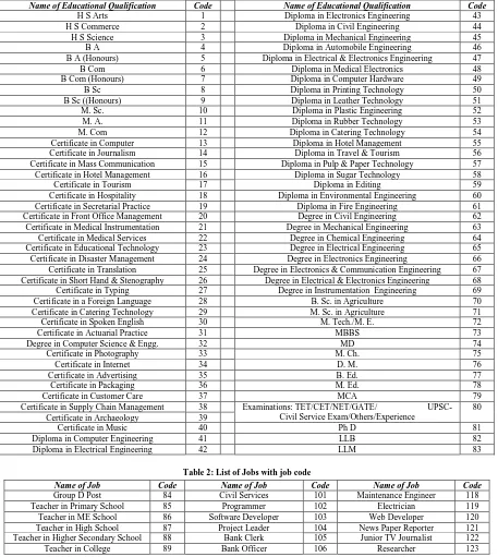
The collected data is preprocessed for mining. The dataset is prepared with 83 different educational qualifications and 49 different job titles. Based on the requirements of various educational qualifications for jobs the transaction dataset for association rule mining is prepared with qualification code and job code on the items in such a way that the job code appears as the last item in the transactions. Item codes in the transactions are also kept sorted in the ascending order. In this way the semantics of the transactions are prepared. The attributes of the data set are shown in tables 1 and 2 below.

Table 1: Educational Qualifications and Respective Codes

Name of Educational Qualification Code Name of Educational Qualification Code

H S Arts 1 Diploma in Electronics Engineering 43 H S Commerce 2 Diploma in Civil Engineering 44 H S Science 3 Diploma in Mechanical Engineering 45 B A 4 Diploma in Automobile Engineering 46 B A (Honours) 5 Diploma in Electrical & Electronics Engineering 47 B Com 6 Diploma in Medical Electronics 48 B Com (Honours) 7 Diploma in Computer Hardware 49 B Sc 8 Diploma in Printing Technology 50 B Sc ((Honours) 9 Diploma in Leather Technology 51 M. Sc. 10 Diploma in Plastic Engineering 52 M. A. 11 Diploma in Rubber Technology 53 M. Com 12 Diploma in Catering Technology 54 Certificate in Computer 13 Diploma in Hotel Management 55 Certificate in Journalism 14 Diploma in Travel & Tourism 56 Certificate in Mass Communication 15 Diploma in Pulp & Paper Technology 57 Certificate in Hotel Management 16 Diploma in Sugar Technology 58 Certificate in Tourism 17 Diploma in Editing 59 Certificate in Hospitality 18 Diploma in Environmental Engineering 60 Certificate in Secretarial Practice 19 Diploma in Fire Engineering 61 Certificate in Front Office Management 20 Degree in Civil Engineering 62 Certificate in Medical Instrumentation 21 Degree in Mechanical Engineering 63 Certificate in Medical Services 22 Degree in Chemical Engineering 64 Certificate in Educational Technology 23 Degree in Electrical Engineering 65 Certificate in Disaster Management 24 Degree in Electronics Engineering 66 Certificate in Translation 25 Degree in Electronics & Communication Engineering 67 Certificate in Short Hand & Stenography 26 Degree in Electrical & Electronics Engineering 68 Certificate in Typing 27 Degree in Instrumentation Engineering 69 Certificate in a Foreign Language 28 B. Sc. in Agriculture 70 Certificate in Catering Technology 29 M. Sc. in Agriculture 71 Certificate in Spoken English 30 M. Tech./M. E. 72 Certificate in Actuarial Practice 31 MBBS 73 Degree in Computer Science & Engg. 32 MD 74 Certificate in Photography 33 M. Ch. 75 Certificate in Internet 34 D. M. 76 Certificate in Advertising 35 B. Ed. 77 Certificate in Packaging 36 M. Ed. 78 Certificate in Customer Care 37 MCA 79 Certificate in Supply Chain Management 38 Examinations: TET/CET/NET/GATE/

UPSC-Civil Service Exam/Others/Experience

80 Certificate in Archaeology 39

Certificate in Music 40 Ph D 81 Diploma in Computer Engineering 41 LLB 82 Diploma in Electrical Engineering 42 LLM 83

Table 2: List of Jobs with job code

Name of Job Code Name of Job Code Name of Job Code

Teacher in University 90 Bank Manager 107 Architect 124 Doctor in Medical College 91 Engineer 108 Middle Level Hotel Job 125 Doctor by Profession 92 Junior Engineer 109 Hotel Manager 126 Group C Post 93 Senior Engineer 110 Data Entry Operator 127 Group B Post 94 Paramedical Staff 111 Senior TV Journalist 128 Group A Post 95 Technical Support Staff 112 Middle level Job in police 129 Scientist 96 Hospital Attendant 113 Junior Hotel Job 130 Technician 97 Pharmacist 114 Front Office Operator 131 Technical Supervisor 98 Cashier in Bank 115 Lawyer 132

News Paper Editor 99 Network Engineer 116 Junior/Sub Editor of News Paper 100 Computer Science Teacher 117

Then the a priori algorithm is implemented with T – Tree as the internal data structure for discovering the association rules showing eligibility for jobs. Then from the transaction data set of eligibility for jobs, the frequent itemsets are generated with respect to a pre specified value of minimum support. The association rules with respect to the pre specified minimum support and minimum confidence are generated from the frequent itemsets in such a way that the name of the job occurs in the consequent and all the required qualifications appear in the antecedent of the rules of the form X→Y where X represents the set of qualifications for the job represented by Y. This is the additional condition applied on the consequents of the rules and only the required rules are considered. The results are interpreted after analysis and conclusion is drawn.

This approach helps the candidates to find suitable employment options based on their qualifications in the form of association rules.

Thereafter, different sets of qualifications required for a job are identified from the large number of discovered rules by grouping the discovered association rules for the same job.

Candidates with a specific set of qualifications are also eligible for different jobs. For this the association rules with same qualifications appearing on the antecedent and different jobs on the consequent are identified and grouped.

IV. THE A PRIORI ALGORITHM

The A priori algorithm uses the downward closure property which states that any subset of a frequent itemset is a frequent itemset [5] [6]. This means if an itemset is found to be infrequent, then there is no need to generate any superset of this as candidate because it will also certainly be infrequent. This is the upward closure property according to which any superset of an infrequent itemset is infrequent.

The algorithm applies bottom up search and prunes away many of the itemsets which are unlikely to be frequent before reading the database at every level. In this method candidate itemsets of a particular size are generated at first, and then the database is scanned to count their supports to check if they are large.

In the first scan of the database, all itemsets of size-1 are treated as candidate itemsets. These candidate itemsets are

denoted as C1. From these candidate itemsets of size 1 (C1) large itemsets of size 1 denoted as L1 are computed by using the pre specified threshold value of minimum support (minsup). For this the support counts of the candidate itemsets of size 1 (C1) are counted in the first scan to find the large itemsets of size 1 (L1).

Let Ck denotes candidate itemset of cardinality k. During the scan k, at first, candidates of size k (Ck) are discovered. Then by using the pre specified threshold value of minimum support (minsup), the large or frequent itemsets of size k (Lk) are computed. By using these large itemsets found in the scan k, the candidate temsets of size (k+1) for the (k+1)th scan of the database are computed. If all the subsets of an itemset are found to be large, then only such an itemset is considered to be a candidate itemset.

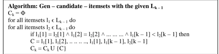
To generate candidates of size k+1, the set of frequent itemsets found in the previous pass, Lk-1, is joined with itself to determine the candidates. An algorithm called A priori – Gen is used to generate candidate itemsets for each pass after the first.

An itemset of size k can be combined with another itemset of the same size if they have (k-1) common items between them. At the end of the first scan, for generating the candidate itemsets of size 2 (C2) every large itemset of size 1 is combined with every other large itemset.of size l.

A subsequent pass, say pass k, consists of two phases: First, the frequent itemsets Lk-1 found in the (k-1)

th

pass (k>1) are used to generate the candidate itemsets Ck using the a priori generation procedure described below. Next the database is scanned and the support of each candidate in Ck is counted. The set of candidate itemsets is subjected to a pruning process to ensure that all the subsets of the candidate sets are frequent itemsets.

The candidate generation and the pruning processes are discussed below. The A priori algorithm assumes that the data base is memory resident. The maximum number of database scans is one more than the cardinality of the largest frequent itemset.

Candidate Generation: Given Lk – 1

It is known that if X is a large itemset than all the subsets of X are also large. For example, consider a set of large itemsets of size 3 (L

, the set of all frequent (k – 1) itemsets (k>1), it is required to generate supersets of the set of all frequent (k – 1) itemsets.

3) given as {{a, b, c}, {a, b, e}, {a, c, e}, {b, c, e}, {b, c, d}}. Then the Candidate - 4 itemsets (C4

generated are the supersets of these Large – 3 itemsets (L )

3) and in addition all the 3 – itemset subsets of any candidate – 4 itemset (so generated) must be already known to be in L3. The first part and the part of the second part are handled by A priori candidate generation method.

C4 = {{a, b, c, e}, {b, c, d, e}} is obtained from L3 = {{a, b, c}, {a, b, e}, {a, c, e}, {b, c, e}, {b, c, d}}. {a, b, c, e} is generated from {a, b, c} and {a, b, e}. Similarly, {b, c, d, e} is generated from {b, c, d} and {b, c, e}.

Pruning: Pruning is done to eliminate such candidate itemsets for which all its subsets are not large or frequent. That is, a candidate set is considered to be acceptable if all its subsets are frequent. For example, from C4, the itemset {b, c, d, e} is pruned, since all its 3 – subsets are not in L3 (clearly, {b, d, e} is not in L3. The pruning algorithm is described below.

These two functions – candidate generation and pruning are used by the a priori algorithm in every iteration. It moves

upward in the lattice starting from level 1 to level k, where no candidate set remains after pruning.

The a priori algorithm is applied on the experimental dataset prepared and various results are obtained. These results are presented in the next section.

Below, the working of the a priori algorithm is shown on the sample dataset of Table 5 for the discovery of the association rules for mining the eligibility criteria for jobs. The pre specified minimum support (minsup) is assumed to

be minsup=1/30 = 0.033 = 3.3% i.e. minimum support count = 1.

The attributes (items) of the sample data set for this example is drawn from the tables 1 and 2 above based on the survey carried out and are shown in table 3 and table 4 respectively. The sample data set for this example is drawn from the survey carried out and is shown in table 5 below.

Table 3: List of Eligibility Qualifications and names of jobs with codes

Name of Educational Qualification

Code Name of Educational Qualification

Code Name of Educational Qualification Code

H S Arts 1 B Sc 8 Degree in Chemical Engineering 64 H S Commerce 2 M. Sc. 10 M. Tech./M. E. 72 H S Science 3 M. A. 11 MBBS 73 B A 4 M. Com 12 B. Ed. 77 B Com 6 Degree in Civil Engineering 62 LLB 82

Algorithm: Gen – candidate – itemsets with the given Lk – 1

Ck= Φ

for all itemsets l1ϵ Lk – 1 do for all itemsets l2ϵ Lk – 1 do

if l1[1] = l2[1] ˄ l1[2] = l2[2] ˄ ... ... ... ˄ l1[k – 1] < l2[k – 1] then C = l1[1], l1[2], .. .. .. .., l1[1], l1[k – 1], l2[k – 1]

Ck = Ck U {C}

Prune (Ck)

for all c ϵ Ck

for all (k – 1)- subsets d of c do if d ϵ Lk– 1then Ck = Ck \ {c}

A priori Algorithm

Initialize: k: = 1, C1 = all the 1 – itemsets;

Read the database to count support of C1 to determine L1; L1 = {frequent – 1 itemsets};

k: = 2, // k represents the pass number // while (Lk -1≠ Φ) do

begin

Ck = gen_Candidate_Itemsets with the given Lk -1; prune (Ck) ;

for all transactions t ϵ T do

increment the count of all candidates in t; Lk = All candidates in Ck with minimum support; k: = k + 1;

end;

Table 4: List of Jobs with job code [The list of job codes is taken from [1]]

Job Title Job Code Job Title Job Code Job Title Job Code

Teacher in High School 87 Group B Post 94 Engineer 108 Teacher in Higher Secondary School 88 Group A Post 95 Lawyer 132

Doctor by Profession 92 Scientist 96 Group C Post 93 News Paper Editor 99

Table 5: Sample data set [The sample data set is taken from [1]]

TID Items TID Items TID Items TID Items TID Items

1 1 4 77 87 7 3 62 94 13 1 4 82 132 19 3 8 95 25 1 4 99 2 2 6 77 87 8 3 64 94 14 2 6 82 132 20 3 62 95 26 1 4 11 99 3 3 8 77 87 9 3 62 108 15 3 8 82 132 21 3 64 95 27 1 4 11 77 88 4 1 4 93 10 3 64 108 16 3 73 92 22 3 8 10 95 28 2 6 12 77 88 5 2 6 93 11 3 62 72 96 17 1 4 95 23 1 4 11 95 29 3 8 10 77 88 6 3 8 93 12 3 64 72 96 18 2 6 95 24 2 6 12 95 30 3 73 95

Step 1: Generation of Candidate – 1 Itemsets (C1)

Table 6: Candidate – 1 Itemsets (C1) and all are qualified as Frequent – 1 (F1

with respect to minimum support count = 1 or minsup = 0.033 = 3.3%. ) itemsets

Itemset Support Count

Itemset Support Count

Itemset Support Count

Itemset Support Count

Itemset Support Count

1 8 8 6 64 4 87 3 95 9 2 6 10 2 72 2 88 3 96 2 3 15 11 3 73 2 92 1 99 2 4 8 12 2 77 6 93 3 108 2 6 6 62 4 82 3 94 2 132 3

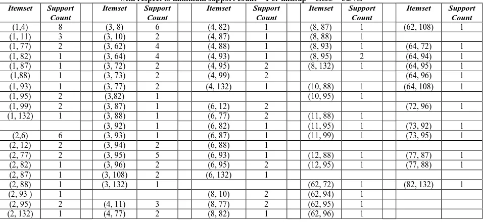
Step 2: Generation of Candidate – 2 Itemsets (C2) with non zero support count and the Frequent – 2 (F2) itemsets

Table 7: Candidate – 2 Itemsets (C2) with non zero support count and all are qualified as Frequent – 2 (F2

with respect to minimum support count = 1 or minsup = 0.033 = 3.3%.

) itemsets

Itemset Support Count

Itemset Support Count

Itemset Support Count

Itemset Support Count

Itemset Support Count

(1,4) 8 (3, 8) 6 (4, 82) 1 (8, 87) 1 (62, 108) 1 (1, 11) 3 (3, 10) 2 (4, 87) 1 (8, 88) 1

(1, 77) 2 (3, 62) 4 (4, 88) 1 (8, 93) 1 (64, 72) 1 (1, 82) 1 (3, 64) 4 (4, 93) 1 (8, 95) 2 (64, 94) 1 (1, 87) 1 (3, 72) 2 (4, 95) 2 (8, 132) 1 (64, 95) 1 (1,88) 1 (3, 73) 2 (4, 99) 2 (64, 96) 1 (1, 93) 1 (3, 77) 2 (4, 132) 1 (10, 88) 1 (64, 108) 1 (1, 95) 2 (3,82) 1 (10, 95) 1

(1, 99) 2 (3, 87) 1 (6, 12) 2 (72, 96) 1 (1, 132) 1 (3, 88) 1 (6, 77) 2 (11, 88) 1

(3, 92) 1 (6, 82) 1 (11, 95) 1 (73, 92) 1 (2,6) 6 (3, 93) 1 (6, 87) 1 (11, 99) 1 (73, 95) 1 (2, 12) 2 (3, 94) 2 (6, 88) 1

(2, 77) 2 (3, 95) 5 (6, 93) 1 (12, 88) 1 (77, 87) 1 (2, 82) 1 (3, 96) 2 (6, 95) 2 (12, 95) 1 (77, 88) 1 (2, 87) 1 (3, 108) 2 (6, 132) 1

(2, 88) 1 (3, 132) 1 (62, 72) 1 (82, 132) 1 (2, 93 ) 1 (8, 10) 2 (62, 94) 1

(2, 95) 2 (4, 11) 3 (8, 77) 2 (62, 95) 1 (2, 132) 1 (4, 77) 2 (8, 82) 1 (62, 96) 1

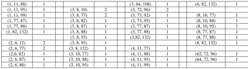
Step 3: Generation of Candidate – 3 Itemsets (C3) with non zero support count and the Frequent – 3 (F3) itemsets

Table 8: Candidate – 3 Itemsets (C3) with non zero support count and all are qualified as Frequent – 3 (F3

with respect to minimum support count = 1 or minsup = 0.033 = 3.3%.

) itemsets

Itemset Support Count

Itemset Support Count

Itemset Support Count

Itemset Support Count

(1, 4, 11) 2 (2, 6, 93 ) 1 (3, 62, 72) 1 (4, 77, 87) 1 (1, 4, 77) 2 (2, 6, 95) 2 (3, 62, 94) 1 (4, 77, 88) 1 (1, 4, 82) 1 (2, 6, 132) 1 (3, 62, 95) 1 (4, 82, 132) 1 (1, 4, 87) 1 (2, 12, 77) 1 (3, 62, 96) 1

(1, 11, 88) 1 (3, 64, 108) 1 (6, 82, 132) 1 (1, 11, 95) 1 (3, 8, 10) 2 (3, 72, 96) 2

(1, 11, 99) 1 (3, 8, 77) 2 (3, 73, 92) 1 (8, 10, 77) 1 (1, 77, 87) 1 (3, 8, 82) 1 (3, 73, 95) 1 (8, 10, 88) 1 (1, 77, 88) 1 (3, 8, 87) 1 (3, 77, 87) 1 (8, 10, 95) 1 (1, 82, 132) 1 (3, 8, 88) 1 (3, 77, 88) 1 (8, 77, 87) 1 (3, 8, 93) 1 (3,82, 132) 1 (8, 77, 88) 1 (2, 6, 12) 2 (3, 8, 95) 1 (8, 82, 132) 1 (2, 6, 77) 2 (3, 8, 132) 1 (4, 11, 77) 1

(2,6, 82) 1 (3, 10, 77) 1 (4, 11, 88) 1 (62, 72, 96) 1 (2, 6, 87) 1 (3, 10, 88) 1 (4, 11, 95) 1 (64, 72, 96) 1 (2, 6, 88) 1 (3, 10, 95) 1 (4, 11, 99) 1

Step 4: Generation of Candidate – 4 Itemsets (C4) with non zero support count and the Frequent – 3 (F4) itemsets

Table 9: Candidate – 4 Itemsets (C4) with non zero support count and all are qualified as Frequent – 4 (F4

with respect to minimum support count = 1 or minsup = 0.033 = 3.3%.

) itemsets

Itemset Support Count

Itemset Support Count

Itemset Support Count

Itemset Support Count

(1, 4, 11, 77) 1 (1, 11, 77, 88) 1 (3, 8, 10, 77) 1 (3, 8, 10, 95) 1 (1, 4, 11, 95) 1 (2, 6, 12, 77) 1 (3, 8, 77, 88) 1 (3, 10, 77, 88) 1 (1, 4, 11, 99) 1 (2, 6, 12, 88) 1 (3, 8, 82, 132) 1 (3, 62, 72, 96) 1 (1, 4, 11, 88) 1 (2, 6, 12, 95) 1 (3, 8, 77, 87) 1 (3, 64, 72, 96) 1 (1, 4, 77, 87) 1 (2, 6, 77, 87) 1 (3, 8, 77, 88) 1 (6, 12, 77, 88) 1 (1, 4, 77, 88) 1 (2, 6, 77, 88) 1 (3, 8, 82, 132) 1 (8, 10, 77, 88) 1 (1, 4, 82, 132) 1 (2,6, 82, 132) 1 (3, 8, 10, 77) 1

(1, 4, 11, 99) 1 (2, 12, 77, 88) 1 (3, 8, 10, 88) 1

Step 5: Generation of Candidate – 5 Itemsets (C5) with non zero support count and the Frequent – 3 (F5) itemsets

Table 10: Candidate – 5 Itemsets (C5) with non zero support count and all are qualified as Frequent – 5 (F5

with respect to minimum support count = 1 or minsup = 0.033 = 3.3%.

) itemsets

Itemset Support Count Itemset Support Count Itemset Support Count

(1, 4, 11, 77, 88) 1 (2, 6, 12, 77, 88) 1 (3, 8, 10, 77, 88) 1

V. IMPLEMENTATION

The a priori algorithm is implemented on a PC with core 2 duo processor with 1 GB RAM and 100 GB hard disk capacity on windows. The programs are written in Java (JDK 1.2) with T Tree as the underlying data structure.

The data are collected based on a survey conducted among the employed people in various organizations and then the data set is prepared in the transaction format. The steps of the experimentation are as below:

1. The frequent itemsets with respect to a pre specified minimum support (minsup) are discovered. Then those frequent item sets having one item belonging to the list of jobs in table 2 are considered. (No transaction has two items from the table 2 (List of Jobs with job code).

2. Then the association rules are generated with respect to a pre specified minimum support (minsup) and minimum confidence (minconf) and only those discovered association rules are considered which are having only a single item in the consequent and which belongs to the list of jobs in table 2. These rules are analyzed to find the different sets of qualifications required for a job for the pre specified support and confidence.

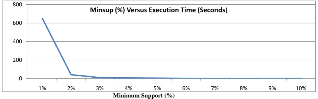
3. The computing time for the discovery of the rules are plotted for different values of support for the data set of the same size.

4. Frequent itemsets, frequent Itemsets having its last item as job code, the association rules and the

Association Rules whose consequent is a job code are discovered from the Job Eligibility Dataset by varying the pre specified minimum support threshold (minsup) at fixed value of confidence (minconf) 1% and corresponding graphs are plotted.

5. Frequent itemsets, frequent Itemsets having its last item as job code, the association rules and the association rules whose consequent is a job code are discovered from the job eligibility dataset by varying the pre specified minimum confidence (minconf) threshold at fixed value of pre specified minimum support(minsup) 3% and corresponding graphs are plotted.

6. By varying the size of the dataset at specific values of pre specified support and confidence the scalability of the algorithm is tested by computing and plotting the computational time of the implementation.

7.

A. The Experimental Set up

The experimental set up after the collection of data is depicted in figure 1 and has the following steps

2. Implement the a priori algorithm with T – Tree as the internal data structure.

3. Discover the association rules.

4. Classify the rules and conclude the discovery with interpretation.

Figure 1: Experimental Steps

VI. EXPERIMENTAL RESULTS

Several results are obtained from the experiments performed and these are described and analyzed in this section

.

A. Experimental Result 1

Frequent Itemsets and the association rules are discovered from the Job Eligibility Dataset by varying the pre specified minimum support threshold (minsup) at fixed value of confidence (minconf). Then the frequent itemsets having the last item belonging to the list of jobs are considered relevant and their numbers at each value of minsup is found. Then such frequent itemsets are plotted against all the frequent itemsets at different values of minsup for a specific value of minconf (Figure 2). Similarly, the association rules having only a job

code as consequent are considered relevant and their numbers at each value of minsup is found and plotted against all association rules discovered (Figure 3). The execution times are also noted and plotted with respect to the various minsup (Figure 4). In Table 11, the frequent itemsets discovered with respect to various values of pre specified minimum support (minsup) at a fixed value of pre specified minimum confidence (minconf) 1% are shown. Then only the frequent itemsets having its last item as job code in the list of jobs are considered. Similarly only the association rules with a job code as its consequent from the list of jobs are retained. As can be seen from table 11, the lower the value of pre specified minimum support the more is the number of association rules discovered..

Table 11: Frequent itemsets, frequent Itemsets having its last item as job code, the association rules and the Association Rules whose consequent is a job code are discovered from the Job Eligibility Dataset by varying the pre specified

minimum support threshold (minsup) at fixed value of confidence (minconf) 1%.

Discovering Frequent Itemsets and association rules at varying pre specified minimum support (minsup) and fixed pre specified minimum confidence (minconf) of 1%

Data Set: Job EligibilityData Set.dat (11KB)(1000 lines) S.

No

Minimum support (minsup) (%)

No. of Frequent Itemsets

No. of Frequent Itemsets having its last

item as job code

No. of Association

Rules

No. of Association Rules whose consequent is a job

code

Execution Time (Seconds)

1 1% 905 412 8616 366 651.706

2 2% 331 106 1900 106 41.075

3 3% 165 28 654 38 9.969

4 4% 112 23 346 27 5.881

5 5% 87 22 238 22 4.275

6 6% 54 8 102 8 2.433

7 7% 39 3 50 3 1.809

8 8% 34 2 41 2 1.763

9 9% 27 1 28 1 1.774

10 10% 25 1 26 1 1.575

Prepare the data collected by survey in a transaction data set format

Implement the a priori algorithm on the transaction data set

Discover the Frequent Item Sets and the Association Rules with respect to pre specified support and confidence

Classify the rules

Interpret the classified rules

Support (%)

Figure 2: Plot of frequent itemsets and frequent Itemsets having its last item as job code discovered from the Job Eligibility Dataset by varying the pre specified minimum support threshold (minsup) at fixed value of confidence (minconf) 1%.

Figure 3: Plot of association rules and the association rules having a job code as consequent discovered from the Job Eligibility Dataset by varying the pre specified minimum support threshold (minsup) at fixed value of confidence (minconf) 1%.

Minimum Support (%)

Figure 4: Variation of execution times with respect to variation in minimum support (%) (minsup)

B. Experimental Result 2

The frequent itemsets and the association rules at varying pre specified minimum confidence (minconf) and at fixed pre specified minimum support (minsup) are discovered form the job eligibility dataset. Then the number of frequent itemsets having its last item as job code and the association rules

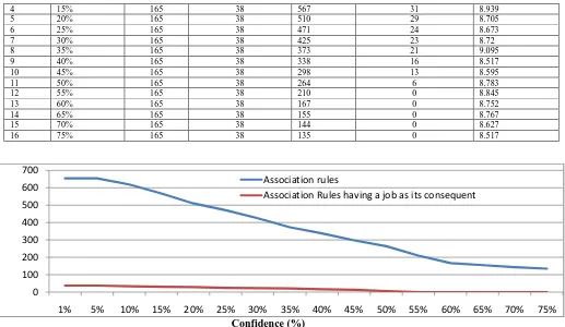
whose consequent is a job code are discovered from the job eligibility dataset by varying the pre specified minimum confidence (minconf) threshold at fixed value of pre specified minimum support(minsup). The execution times are recorded. These results are shown at Table 12. These are plotted in figures 5 and figure 6 respectively.

Table 12: Frequent itemsets, frequent Itemsets having its last item as job code, the association rules and the association rules whose consequent is a job code are discovered from the job eligibility dataset by varying the pre specified minimum confidence (minconf) threshold at fixed value of pre specified minimum support (minsup) 3%.

Discovering Frequent Itemsets and association rules at varying pre specified minimum confidence (minconf) and fixed pre specified minimum support (minsup)of 3% . Data Set: Job EligibilityData Set.dat (11KB) (1000 lines)

S. No Minimum confidence (minconf) (%)

No. of Frequent

Itemsets

No. of Frequent Itemsets having its last item as job code

No. of Association

Rules

No. of Association Rules whose consequent is a job code

Execution Time (Seconds)

1 1% 165 38 654 38 8.768

2 5% 165 38 654 38 9.032

3 10% 165 38 619 34 8.767

0 200 400 600 800 1000

1% 2% 3% 4% 5% 6% 7% 8% 9% 10%

F1: Frequent Itemsets

F2: Frequent Itemsets having its last item as job code

0 2000 4000 6000 8000 10000

1% 2% 3% 4%

A1: Association rules

A2: Association rules with a job code as consequent

0 200 400 600 800

1% 2% 3% 4% 5% 6% 7% 8% 9% 10%

4 15% 165 38 567 31 8.939

5 20% 165 38 510 29 8.705

6 25% 165 38 471 24 8.673

7 30% 165 38 425 23 8.72

8 35% 165 38 373 21 9.095

9 40% 165 38 338 16 8.517

10 45% 165 38 298 13 8.595

11 50% 165 38 264 6 8.783

12 55% 165 38 210 0 8.845

13 60% 165 38 167 0 8.752

14 65% 165 38 155 0 8.767

15 70% 165 38 144 0 8.627

16 75% 165 38 135 0 8.517

Confidence (%)

Figure 5: variation of number of association rules and the association rules whose consequent is a job code with variation in the pre specified minimum confidence (minconf) threshold at fixed value of pre specified minimum support(minsup) 3%.

Figure 6: Execution time (Seconds) with variation in the pre specified minimum confidence (minconf) threshold at fixed value of pre specified minimum support (minsup) 3%.

C. Experimental Result 3

In the Table 13, some of the association rules discovered having only a single item in the consequent belonging to the

list of jobs in Table 2 of the Job Eligibility Dataset are shown with their meaning along with support and confidence. It is not

possible to show all such discovered rules for different combinations of support and confidence. Here only the association rules whose consequent is a job code are shown at fixed value of pre specified minimum support(minsup) 3% and pre specified minimum confidence (minconf) threshold 1%. Similarly, such association rules can be discovered for various values of pre specified minimum support (minsup).

Table 13: Some of the discovered association rules having only a single item in the consequent belong to the list of jobs in table 2 of the Job Eligibility Dataset are shown with their meaning along with support and confidence.

S. No. Association Rule with a job code

in the consequent

Meaning of the Rule Support

(%)

Confidence (%) Qualifications in the antecedent Name of the Job with basic

Qualification

1 [1]--->[132] HS Arts Lawyer with HS in Arts 3.2% 11.594203 2 [2]--->[109] H S Commerce Junior Engineer with HS in Commerce 3.3% 17.460318 3 [3]--->[101] H S Science Civil Services with HS in Science 4.4% 8.224299 4 [3]--->[108] H S Science Engineer with HS in Science 3.7% 6.915888 5 [3]--->[109] H S Science Junior Engineer with HS in Science 5.0% 9.345795

0 100 200 300 400 500 600 700

1% 5% 10% 15% 20% 25% 30% 35% 40% 45% 50% 55% 60% 65% 70% 75%

Association rules

Association Rules having a job as its consequent

8.2 8.4 8.6 8.8 9 9.2

1% 5% 10% 15% 20% 25% 30% 35% 40% 45% 50% 55% 60% 65% 70% 75%

Execution Time (Sec)

6 [80]--->[101] Examinations: TET/CET/NET/GATE UPSC- Civil Service Exam/Others/Experience

Civil Services with UPSC- Civil Service Exam

4.8% 13.483146

7 [82]--->[132] LLB Lawyer with LLB 7.3% 37.2449 8 [83]--->[132] LLM Lawyer with LLM 3.9% 24.074074 9 [3]--->[89] H S Science Teacher in College with HS in Science 5.1% 9.53271 10 [80]--->[89] Examinations:

TET/CET/NET/GATE/UPSC-Civil Service Exam/Others/Experience

Teacher in College with NET/GATE 8.8% 24.7191

11 [81]--->[89] Ph D Teacher in College with Ph. D 5.0% 42.016808 12 [82]--->[89] LLB Teacher in College with LLB 5.9% 30.102041 13 [83]--->[89] LLM Teacher in College with LLM 5.9% 36.419754 14 [3]--->[90] H S Science Teacher in University with HS in

Science

10.0% 12.149532

15 [80]--->[90] Examinations: TET/CET/NET/GATE UPSC-Civil Service Exam/Others/Experience

Teacher in University with NET/GATE 3.0% 28.089888

16 [81]--->[90] Ph D Teacher in University with Ph. D. 5.9% 49.57983 17 [82]--->[90] LLB Teacher in University with LLB 6.4% 32.65306 18 [83]--->[90] LLM Teacher in University with LLM 6.4% 39.506172 19 [3, 80]--->[101] H S Science, Examinations:

TET/CET/NET/GATE/ UPSC-Civil Service Exam/Others/Experience

Civil Services with H S Science, UPSC-Civil Service Exam

4.4% 19.81982

20 [1, 82]--->[132] HS Arts, LLB Lawyer with HS Arts, LLB 3.2% 44.444443 21 [82, 83]--->[132] LLB, LLM Lawyer with LLB, LLM 3.9% 24.074074 22 [3, 80]--->[89] H S Science, Examinations:

TET/CET/NET/GATE/ UPSC-Civil Service Exam/Others/Experience

Teacher in College with H S Science, NET/GATE

4.8% 21.621622

23 [80, 81]--->[89] Examinations: TET/CET/NET/GATE/UPSC-Civil Service Exam/Others/Experience, Ph D

Teacher in College with NET/GATE, Ph D

4.5% 41.284405

24 [80, 82]--->[89] Examinations: TET/CET/NET/GATE/UPSC-Civil Service Exam/Others/Experience, LLB

Teacher in College with NET, LLB 5.3% 47.74775

25 [80, 83]--->[89] Examinations: TET/CET/NET/GATE/UPSC-Civil Service Exam/Others/Experience, LLM

Teacher in College with NET, LLM 5.3% 47.74775

26 [82, 83]--->[89] LLB, LLM Teacher in College with LLB, LLM 5.9% 36.419754 27 [3, 80]--->[90] H S Science, Examinations:

TET/CET/NET/GATE/ UPSC-Civil Service Exam/Others/Experience

Teacher in University with H S Science, NET/GATE

6.2% 27.927927

28 [3, 81]--->[90] H S Science, Ph D Teacher in University with H S Science, Ph D

3.5% 49.295776

29 [80, 81]--->[90] Examinations: TET/CET/NET/GATE/UPSC-Civil Service Exam/Others/Experience, Ph D

Teacher in University with NET/GATE, Ph D

5.4% 49.541283

30 [80, 82]--->[90] Examinations: TET/CET/NET/GATE/UPSC-Civil Service Exam/Others/Experience, LLB

Teacher in University with NET, LLB 5.8% 52.25225

31 [81, 82]--->[90] Ph D, LLB Teacher in University with Ph D, LLB 3.0% 52.63158 32 [80, 83]--->[90] Examinations:

TET/CET/NET/GATE/UPSC-Civil Service Exam/Others/Experience, LLM

Teacher in University with NET, LLM 5.8% 52.25225

33 [81, 83]--->[90] Ph D, LLM Teacher in University with Ph D, LLM 3.0% 52.63158 34 [82, 83]--->[90] LLB Teacher in University with LLB 6.4% 39.506172 35 [80, 82,

83]--->[89]

Examinations: TET/CET/NET/GATE/UPSC-Civil Service Exam/Others/Experience, LLB, LLM

Teacher in College with NET, LLB, LLM

5.3% 47.74775

36 [3, 80, 81]--->[90]

H S Science, Examinations: TET/CET/NET/GATE/ UPSC-Civil Service Exam/Others/Experience, Ph D

Teacher in University with H S Science, NET/GATE, Ph D

3.2% 49.23077

37 [80, 82, 83]--->[90]

H S Science, Examinations: TET/CET/NET/GATE/ UPSC-Civil Service Exam/Others/Experience, LLB, LLM

Teacher in University with H S Science, NET, LLB, LLM

5.8% 52.25225

38 [81, 82, 83]--->[90]

Ph D, LLB, LLM Teacher in University with Ph D, LLB, LLM

3.0% 52.63158

It is observed from Table 13 that in the case of many rules with the same consequent their antecedents are proper subsets of the antecedents of some other rules in the list. This means that a rule with larger set of elements in antecedent specifies all the required and desired qualifications for a particular job. As a result all such rules in which their antecedents are proper subset of the antecedent of another rule can be treated as redundant and can therefore be filtered out. For example, from table 14, consider the rules [1]--->[132] , [82]--->[132] , [83]--->[132], and [1, 82]--->[132]. In these rules, the two rules [1]--->[132] , [82]--[1]--->[132] can be treated as redundant as their antecedents are proper subsets of the rule [1, 82]--->[132]. Therefore, these two rules can be filtered out. The reason for this is that the information obtained from the rules [1]--->[132]

, [82]--->[132] is included in the rule [1, 82] --->[132] and so it is more complete as compared to the two rules. However, the rules [1]--->[132] and [83]--->[132] are also informative to a certain extent as these contain only a single qualification in

their antecedents for the job specified by its consequent. All such rules are discovered as these rules satisfy the pre specified thresholds on minimum support and confidence.

Formally, in the table 14, if there are association rules say X1 →Y, X2 →Y, …., Xn → Y and X → Y such that X1 X, X2

information with their support and confidence. The rules obtained based on this criterion are shown in Table 14 below.

D. Experimental Result 4

A classification of the association rules discovered after mining are done for analyzing the background qualifications required for various jobs is shown in Table 15.

Table 14: Some of the discovered association rules having only a single item in the consequent belong to the list of jobs in table 2 of the Job Eligibility Dataset and satisfying the criterion: if X1→Y, X2→Y, …., Xn

X

→ Y and X → Y are association rules such that

1 X, X2 X , …, and Xn X then only the rule X → Y is considered with its meaning and support and confidence.

S. No.

Association Rule with a job code in the consequent

Meaning of the Rule Suppor

t (%)

Confidence (%) Qualifications in the antecedent Name of the Job with basic

Qualification

1 [2]--->[109] H S Commerce Junior Engineer with HS in Commerce

3.3% 17.460318

2 [3]--->[108] H S Science Engineer with HS in Science 3.7% 6.915888 3 [3]--->[109] H S Science Junior Engineer with HS in Science 5.0% 9.345795 4 [3, 80]--->[101] H S Science, Examinations: TET/CET/NET/GATE/

UPSC-Civil Service Exam/Others/Experience

Civil Services with H S Science, UPSC-Civil Service Exam

4.4% 19.81982

5 [1, 82]--->[132] HS Arts, LLB Lawyer with HS Arts, LLB 3.2% 44.444443 6 [82,

83]--->[132]

LLB, LLM Lawyer with LLB, LLM 3.9% 24.074074

7 [3, 80]--->[89] H S Science, Examinations: TET/CET/NET/GATE/ UPSC-Civil Service Exam/Others/Experience

Teacher in College with H S Science, NET/GATE

4.8% 21.621622

8 [80, 81]--->[89] Examinations: TET/CET/NET/GATE/ UPSC-Civil Service Exam/Others/Experience, Ph D

Teacher in College with NET/GATE, Ph D.

4.5% 41.284405

9 [80, 82]--->[89] Examinations: TET/CET/NET/GATE/ UPSC-Civil Service Exam/Others/Experience, LLB

Teacher in College with NET, LLB 5.3% 47.74775

10 [80, 83]--->[89] Examinations: TET/CET/NET/GATE/UPSC-Civil Service Exam/Others/Experience, LLM

Teacher in College with NET, LLM

5.3% 47.74775

11 [82, 83]--->[89] LLB, LLM Teacher in College with LLB, LLM 5.9% 36.419754 12 [80, 82,

83]--->[89]

Examinations: TET/CET/NET/GATE/ UPSC-Civil Service Exam/Others/Experience,

LLB, LLM

Teacher in College with NET, LLB, LLM

5.3% 47.74775

13 [3, 80, 81]--->[90]

H S Science, Examinations: TET/CET/NET/GATE/ UPSC-Civil Service Exam/Others/Experience, Ph D

Teacher in University with H S Science, NET/GATE, Ph D

3.2% 49.23077

14 [80, 82, 83]--->[90]

H S Science, Examinations: TET/CET/NET/GATE/ UPSC-Civil Service Exam/Others/Experience,

LLB, LLM

Teacher in University with H S Science, NET, LLB, LLM

5.8% 52.25225

15 [81, 82, 83]--->[90]

Ph D, LLB, LLM Teacher in University with Ph D, LLB, LLM

3.0% 52.63158

Table 15: Classification of the association rules discovered with minsup =3% and minconf =1%

Name of the Job Background Qualification required

Lawyer HS Arts/HS Science, LLB/ LLM; LLB, LLM Junior Engineer H S Commerce / H S Science

Engineer H S Science

Civil Services H S Science/Arts/Commerce, BA, B.Sc., B. Com, BE, UPSC- Civil Service Exam Teacher in College H S Science/Arts/Commerce, BA, B.Sc., B. Com, LLB, LLM, Ph. D., NET

Teacher in University H S Science/Arts/Commerce, BA, B.Sc., B. Com, LLB, LLM, Ph. D., NET, Examinations: NET/GATE, Ph D.

VII. DISCUSSION AND CONCLUSION

In this paper apriori algorithm is implemented with T Tree to discover the eligibility qualifications required for jobs. A survey was undertaken to collect and prepare the data about employment.

As a future work both association and classification or association and clustering techniques shall be applied in a

hybrid manner for further refinements of the results. Rules can also be grouped by using clustering based on similarity.

All such association rules which show the same eligibility qualification for different jobs are grouped together under a classification scheme and based on the support and confidence of the rules the rules can be ranked. This approach of classification of rules helps in determining the groups of jobs for which the same eligibility criteria are required.

REFERENCES

[1] P. K. Deva Sarma, “An Association Rule Based Model for Discovery of Eligibility Criteria for Jobs”, International Journal of Computer Sciences and Engineering, Vol. 6, No. 2, pp. 143-149, 2018.

[2] M. S. Chen, J. Han, P. S. Yu, “Data Mining: An Overview from a Database Perspective”, IEEE Transactions on

Knowledge and Data Engineering (TKDE), Vol. 8, No. 6, pp. 866-883, 1996

[4] M. J. Zaki, “Scalable Algorithms for Association Mining”, IEEE Transactions on Knowledge and Data Engineering, Vol. 12, No 3, pp. 372 – 390, 2000.

[5] R. Agrawal, T. Imielinsky, and A. Swami, “Mining Association Rules Between Sets of Items in Large Databases”, Proceedings of ACM SIGMOD Intl. Conference on Management of Data, pp. 207 -216, USA, 1993.

[6] R. Agrawal and R. Srikant, “Fast Algorithms for Mining Association Rules in Large Databases”, Proceedings of 20th

[16] A. Savasere, E. Omiecinski, and S. Navathe, “An Efficient Algorithm for Mining Association Rules in Large

Databases”, Proceedings of the 21

International Conference on Very Large Databases, pp. 487 – 499, Santiago, Chile, 1994.

[7] S. Brin, R. Motwani, and C. Silverstein, “Beyond Market Baskets: Generalizing Association Rules to Correlations” Proceedings of the ACM International Conference on Management of Data, pp. 265 -276, 1997.

[8] L. Wang, and C. Yi, “Application of Association Rules Mining In Employment Guidance”, Advanced Materials Research Vols. 479-481, pp 129-132.

[9] A. Gupta, and D. Garg, “Applying Data Mining Techniques in Job Recommender System for Considering Candidate Job Preferences”, In the Proceedings of International Conference on Advances in Computing, Communications and Informatics (ICACCI), pp. 1458- 1465, 2014.

[10] C. Chien, and L. Chen, “Data Mining to Improve Personnel Selection and Enhance Human Capital: A Case Study in High-Technology Industry”, Expert Systems with Applications, Vol. 34, No. 1, pp. 280-290, 2008.

[11] B. Jantawan, and C. Tsai, “The Application of Data Mining to Build Classification Model for Predicting Graduate Employment”, International Journal of Computer Science and Information Security, 2013

[12] T. Mishra, D. Kumar, and S. Gupta, “Students’ Employability Prediction Model through Data Mining”, International Journal of Applied Engineering Research, Volume 11, Number 4, pp 2275-2282, 2016.

[13] M. Sapaat, and A. Mustapha, J. Ahmad, K. Chamili, and R. Muhamad, “A Data Mining Approach to Construct a Graduates Employability Model in Malaysia, ” International Journal of New Computer Architectures and their Applications, Vol. 1, No. 4, pp. 1086-1098, 2011. [14] I. A. Wowczko, “Skills and Vacancy Analysis with Data

Mining Techniques”, Informatics, Vol. 2, pp. 31-49, 2015. [15] N. N. Salvithal, and R.B. Kulkarni, “Appraisal Management

System using Data mining Classification Technique”, International Journal of Computer Applications, Volume 135, No.12, 2016.

st

[17] J.L. Lin and M. H. Dunham, “Mining Association Rules: Anti Skew Algorithms,” 14

International Conference on Very Large Data Bases (VLDB), pp. 432-444, Zurich, Switzerland, 1995.

th

[18] S. S. Yen and A. L. P. Chen, “An Efficient Approach to Discovering Knowledge from Large Databases”, Fourth International Conference on Parallel and Distributed Information Systems, 1996.

International Conference on Data Engineering, 1998.

[19] S. Brin, R. Motowani, J. D. Ullman and S. Tsur, “Dynamic Itemset Counting and Implication Rules for Market Basket Data”, Proceedings of the ACM SIGMOD International Conference on Management of Data, 1997.

[20] Lin D.I., and Kedem Z. M., “Pincer –Search: A New Algorithm for Discovering Maximal Frequent Set”, Sixth International Conference on Extending Database Technology, 1998.

[21] D. Gunopulos, H. Mannila, and S. Saluja, “Discovering All the Most Specific Sentences by Randomized Algorithms”, International Conference on Database Theory, 1997. [22] R. J. Bayardo, “Efficiently Mining Long Patterns from

Databases”, Proceedings of ACM SIGMOD International Conference on Management of Data, pp. 85–93, USA, 1998.

[23] J. Han, J. Pei, and Y. Yin, “Mining Frequent Patterns without Candidate Generation”, Proceedings of the ACM SIGMOD International Conference on Management of Data, USA, 2000.

[24] Rakesh Agrawal, “Parallel Mining of Association Rules”, IEEE Transcations on Knowledge and Data Engineering, Vol. 8, No 6, pp. 962-969, 1996.

[25] H. Toivonen, “Sampling Large Databases for Association Rules”, Proceedings, 22nd

[29] Claudia Marinica and Fabrice Guillet, “Knowledge-Based Interactive Postmining of Association Rules using Ontologies”, IEEE Transactions on Knowledge and Data Eng., vol. 22, No. 6, pp. 784 – 797, 2010.

Conference, very Large Databases, 1996.

[26] P. K. Deva Sarma, A. K. Mahanta, “An Apriori Based Algorithm to Mine Association Rules with Inter Itemset Distance”, International Journal of Data Mining and Knowledge Management Process (IJDKP), Vol. 3, No. 6, pp. 73 – 94, November 2013.

[27] M. Hahsler, C. Buchta, and K. Hornik, “Selective Association Rule Generation,” Computational Statistic, vol. 23, no. 2, pp. 303-315, Kluwer Academic Publishers, 2008. [28] F. Guillet and H. Hamilton, Quality Measures in Data

Mining, Springer, 2007.

AUTHOR’S PROFILE