TWO WAY TRACKER A GIS ANCHORED GRAPH SEARCHING METHOD

DOI: http://dx.doi.org/10.26483/ijarcs.v8i7.4299

Volume 8, No. 7, July

–

August 2017

International Journal of Advanced Research in Computer Science

RESEARCH PAPER

Available Online at www.ijarcs.info

ISSN No. 0976-5697

TWO-WAY-TRACKER- A GIS ANCHORED GRAPH SEARCHING METHOD

Subhadip Boral

Department of Computer Science BarrackporeRastraguruSurendranath College

Barrackpore, India

Sudipta Biswas

Department of Computer Science BarrackporeRastraguruSurendranath College

Barrackpore, India

Abstract: Reaching at the goal node in a connected weighted graph, preferably through the optimal path, starting journey from a given source node, plays an important role in GIS. Because, utilizing GPS enabled devices, to reach at destination, is now a very common practice, without having any prior knowledge about the journey. As number of accidents is increasing on each successive day we should prefer not only the shortest but also the short and safe route. The novel intent of the proposed work is to find the shortest path between two places with most safety. Basically the safety measureshave been granted for journey through ocean, but could easily be applied for roadways also, just by changing the influencing factors. All the possible routes touching different cross points could be viewed as connected weighted graph, where various cross points; including source and destination are the nodes. As the target is to find Optimal and Safest path, so not only the length of edge (i.e. distance between its two end points) but also various factors affecting the safety of the journey plays active role in determination of the edge weight. Computation of path weightage has been executed through Regression Analysis using fifth degree polynomial curve fitting, based on input data from historic/ geographic data. The outcome of the method has been graphically displayed which is not only cheaper with respect to distance traversed but also safer in dodging the presence of hazardous weather. The algorithm is implemented in JAVA platform using NetBeans IDE 8.0.2 and the Experimental Result is shown in GUI. Finally, the present techniques have been compared with various Goal Searching techniques for connected graph such as Generate and Test, Simple Hill Climbing, Steepest Ascent Hill Climbing, Best First Search, Dijkstra’s Method and so on.

Keywords: GIS, Weighted Connected Graph, Goal Searching, Optimal and Safest Path, Regression Analysis, Polynomial Curve fitting, NetBeans IDE.

I. INTRODUCTION

Now the travelers are very free to find their route for avoiding

traffic congestion to reach destination timely. The present work deals with finding route searching procedure in a connected

graph. Here it has been applied for finding the less hazardous

route in the ocean for sailing through, but it could be applied

for any other such applications. Till this twenty first century

ocean is one of the main medium of transport of goods for many countries and multinational companies depending on cargo ships. Not only the cargo ships but also the passenger liners are playing an important role for travelling throughout the world. In addition to adverse weather (such as sea storm, Hurricane, fog, lighting, strong winds etc.) low water depth, presence of iceberg etc. can arouse adverse situation for a mariner while propelling the ships. Many deadly shipwrecks have been occurred, directly or indirectly, by intricate weather conditions, some of which could be avoided by choosing alternative less hazardous route for travelling [3]. For any goal searching algorithm (i.e. to reach to the destination from

source) one of the major concern is to find the shortest route. However, for minimizing the possibility of shipwrecks, here

the basic intension is not to find an Optimal, but as well as the

Safest route between two Points – namely, SOURCE and DESTINATION. There present many connected cross-points through which a number of routes exist between Source and Destination. Thus the entire problem is considered as a Graph (Weighted) Traversal problem, between two given points. For determination of the weight of the edges, not only its length (i.e. distance between its two end points), but also various

influencing parameters (values are determined from various

case study or previous history) are considered. Four different

existing Goal finding Approaches, namely Generate – And – Test, Simple Hill – climbing, Steepest –Ascent Hill Climbing and Best-First Search [1] [2] are applied for the above

mentioned safest route finding purpose and problems in each

cases are observed. Finally, a new technique Two way Tracking (TwT) has been developed to overcome some of the demerits of the existing techniques. While finding the Optimal Safest route, equal importance has given to the distance (has to traverse for reaching destination) and safety measures.

II. THESCHEME

Most of the problems related to journey from one point to another, touching some other intermediate points, could be realized as Goal node searching problem in graph. The same approach has also been incorporated here. Thus Starting point of journey (i.e. Source), Ending point of journey (i.e. Destination), all the intermediate points, touching (some of) which journey has to made; all are represented by nodes of Graph. Similarly, the paths connecting nodes are the edges. As journey could be to any direction via edges, so the graph is undirected one. For determination of the weights of the edges, equal priority has given to both the length of the path (i.e.

distance between two end points) and the influencing factors

affecting the smoothness of travel.

The basic intension of the Shortest Path problem is to find a

cheapest path (cheap in terms of cost or distance) between a Source node and a Goal node traversing through existent edges.

For the present purpose, instead of finding the “Shortest” Path, the “Safest Optimal” Path is being searched for, while traversing from a source node S, to reach a destination node D;

where D ε V(G) and S ε V(G) for an undirected graph G(V,E).

Properties of OR Graph:

In OR Graph, vertex i ε V(G) generated from j ε V(G) will

maintain a PARENT LINK to j. It will help to recover the path from D to S.

Thus for the present considered graph also, a vertex i ε V(G) generated from j ε V(G) will maintain a PARENT LINK to j,

which helps to recover the path from D to S. In the current methodology, two lists are maintained:

One is UNPROCESSED, containing the unvisited nodes and the other is SUCCESSORS, containing the adjacent nodes of any chosen one. Initially, Source node is picked. At each step, the best node n (in terms of cost of reaching) among the adjacent nodes of the presently considered nodes is selected from UNPROCESSED and its SUCCESSORS are generated, iff the node n has not been generated previously. However, if it has already been generated, then after comparing the previous cost from node n to D and the latest cost of the same, the best path is assigned. But in this case, node n is not being

regenerated. In this strategy, the single path generated first from

Source S to Destination D is produced as searching result. Thus the strategy does not imply the fact that, the produced path is the shortest one.

To overcome this problem, the strategy of AND-OR graph has also been considered in addition, where at each vertex possibility of reaching Goal is solved or in other words whose successors are fully traversed to reach the goal and then the algorithm decide which of its successor arcs is the most promising and mark it as part of current node. By following these steps for every node and ultimately for the root node, the best way to reach the goal node is generated.

To get a more detailed overview of the technique adapted,

let us define the following symbols: [3]

 Ri – Symbolize path and enumerated by i.

 Ri(n) – Signifies path from source s to node n and enumerated by i.

 f(n) – Denotes the minimum cost from source s to node n.

 fRi(n) – Cost to reach node n from source s maintaining the path Ri.

 fR(n) – Set of all fRi(n), i.e. set of all possible paths from source s to node n.

 B - It is the solution cost generated by the search technique.

 Bj – Denotes the cost of reaching node j from source s.  The proposed algorithm profess order preserving

hallmark. If R1(n), R2(n) are any two paths from source s to n such that the pointers from n to s lie along the path R1 and R2 and fR1(n)≤fR2(n) and if Ri(k) consists node n then R1(n) will be a part of Ri(k) .

 R1(n) is known to be the path assigned to n at termination if fR1(n) = min fR(n)

Terminating Condition for Goal Searching :

 At any time before the proposed algorithm terminates, there exists on UNPROCESSED list, a node n’ that is on some solution path and for which f(n’)≤B

 Let Rj(D) be the solution path with which the proposed algorithm terminates; then any time before termination, there is an UNPROCESSED node n on Rj(D) for which f(n) = fRj(n).

 If there is a solution path and f is such that fRi(n) is unbounded along any infinite path R, then the proposed algorithm terminates with a solution, i.e. the proposed algorithm is complete.

Reduction of Backtracking:

Here,afunctionSUCCESSORS_LEFT_FOR_EXPLORATION(

Q) has been defined, which returns the number of successors of

node Q, till remaining for be explored (visit). In other words, SUCCESSORS_LEFT_FOR_EXPLORATION(Q)=(Number of adjacent nodes of Q except it’s immediate ancestor from which Q has been succeeded - Number of adjacent nodes of Q has been traversed having Q as their immediate ancestor).

Let B is a node from where BACKTRACKING is to start (i.e. have to move back to some already traversed node) and has to roll back to some already traversed node for further exploration. So, if X is already a traversed node and SUCCESSORS_LEFT_FOR_EXPLORATION(X) > 0 and every node between X and B is of

SUCCESSORS_LEFT_FOR_EXPLORATION(Node)=0, then we can directly JUMP to X from B skipping all the nodes in between.

Elaboration of the Backtracking Reduction Process:

Case Study 1: Following figure (Figure 1) shows a graph G1 in which the node X is of degree > 0 and the node B is of SUCCESSORS_LEFT_FOR_EXPLORATION(B) = 3.

After exploration of node B

SUCCESSORS_LEFT_FOR_EXPLORATION(B) will

become 0 and for BACKTRACKING, a direct JUMP to node X could be made without exploring any other nodes lying in between as because for all thenodes between X and B SUCCESSORS_LEFT_FOR_EXPLORATION(Node)=0

If there are m nodes of degree 2 lying between X and B and n is the total number of vertices in the graph then m(n-1) unit time due to adjacency checking during BACKTRACKING could be saved, by incorporating the mentioned methodology.

Figure 1: Case Study 1 (Graph G1)

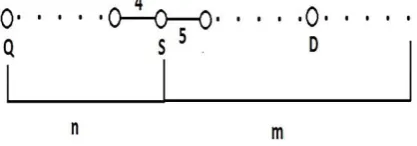
Case Study 2:G2 (Figure 2) is a linear graph where the source node S is of degree 2 and the destination node D is at any side of the source node and D is either of degree 2 or 1. If the lower cost path exists on the opposite side of the destination node (here it is of cost 4) then at first traversal will made to the opposite side of the destination node D up to node Q, from there a direct jump to node S is made, incorporating. During the BACKTRACKING it has to check adjacency (n-2) (n+m-1) times. But with incorporated methodology of direct JUMP from node Q to S (as all the

intermediate nodes have

SUCCESSORS_LEFT_FOR_EXPLORATION(Node) =

0), it could be done in 1 unit time

Incorporation of Two-way-Tracking:

To make the searching procedure even faster, concept of Two-way-Tracking has been incorporated. To implement the concept of TWO-WAY SEARCH, two searching processes- one originated from the SOURCE node and the other one from the DESTINATION node, executed in parallel. In the searching process triggered from SOURCE, the process will try to reach the DESTINATION. Similarly, the searching process triggered from DESTINATION, it will try to reach the SOURCE. The whole procedure will terminate when any of the process able to achieve its goal successfully or meet one another in midway. Both of the searching process maintain their own UNPROCESSED, PROCESSED and PARENT list.

When the searching process PS, triggered from SOURCE, will progress to a node P then it will check whether P is in the PROCESSED list of process PD, searching triggered from DESTINATION, or not. If P is not in the PROCESSED list of PD then no action will be taken. But if it is in the PROCESSED list of PD and PARENT of P is not initialized then using PARENT list of PD, process PS will reach its GOAL node (i.e. node being searched for). When PARENT of P is already initialized then it will check whether progressing in the path maintaining the PARENT list of PD towards the

GOAL is beneficial or not for every intermediate nodes in between P and GOAL along with GOAL node by means of

optimal path generation. If following the path is beneficial

then it will follow the path generated by PD in opposite direction otherwise the consideration of the generated path by PD will be stopped.

The whole procedure, in a similar way, will also be maintained by process PD and it will reach its GOAL node following the same procedure.

Elaboration of the Two-way-Tracking Process:

Case Study 1: Following figure (Figure 3) shows a graph G4 in which the node K is an intermediate node between S, source and D, Destination and exploring K by PS and PD and maintaining PARENT list of PD and PARENT list of PS

respectively will be beneficial. But exploring M and

maintaining PARENT list of PD is not beneficial as PS will be follow parent of M in PARENT list of PS then which is not desirable.

Figure 3: Case Study 1 (Graph G4)

Case Study 2: Following figure (Figure4) PS will follow the path S-C-A-K-D and it will update the parent of K. But exploring path S-C-B-K and following PARENT list of PD in

opposite direction finding K in the PARENT list of PD is not beneficial as maintaining the path will not follow the theory of

optimality.

Figure 4: Case Study 1 (Graph G5)

Maintenance of UNPROCESSED and PROCESSED list:

Let S is a vertex and it have n adjacent vertices and there

are total N nodes in the graph. So for first time S will check

adjacency with (N-1) nodes and it may traverse to node i, i ε n, total number of adjacent vertices of S, and after full exploration of i it will return to S and check adjacency with (N-1) node for next successor j, j ε n and j 6= i and so on. So for n times, at S the algorithm has to check adjacency for n(N-1) times. But if we implement UNPROCESSED list using a LAST-IN-FIRST-OUT principle and insert adjacent node id in monotonic decreasing order by means of their cost then after full exploration of the node being at the TOP of the list, it will be released and the next item will be traversed. Thus by incorporating this methodology, checking adjacencies for n(N-1) times is eliminated, instead it is being done only N times. Here, after fetching and fully exploring node i, the algorithm will automatically progress to node j.

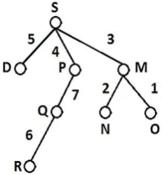
Let us consider the graph G3 shown in Figure 5, in which

S is the source node and D is destination node. At first, S will

check adjacency with all other seven nodes and only the adjacent nodes will be inserted in the following manner: D, P, M (as the path connecting M is of least cost, so M is at TOP). After full exploration of M (i.e. visiting N and O), the process will not move back to S, instead M will be removed from the list, so that P will be the TOP and will be considered next.

The proposed Algorithm of Two-way-Tracking thus could be summarized as follows:

1. Initialize CURRENT node = SOURCE node 2. Insert CURRENT node in UNPROCESSED list 3. If UNPROCESSED list is NOT EMPTY Then

(i) If there are no SUCCESSOR to be traversed or CURRENT node is GOAL node Then

(a) CURRENT node = LAST node in the PROCESSED list

(b) Remove LAST node from PROCESSED list

(ii) Else

(a) Insert all the remaining SUCCESSOR in UNPROCESSED list in ascending order in terms of cost

(b) Select the BEST node from the remaining SUCCESSOR to be traversed (c) If the number of remaining SUCCESSOR is > 1

• Insert CURRENT node in the

PROCESSED list (d) End If

(iii) Remove CURRENT node from

UNPROCESSED list

(iv) CURRENT node = BEST node (v) End If

(vi) Goto 3 4. End If

5. End.

Influencing Criteria of the Route:

While searching for the safest route at first it is needed to find the factors influencing the safety of the route. These

factors vary from application to application (i.e. factors changes if being shifted from route through ocean to route through roadways). As here, safest route for sailing through

ocean is targeted; among a lot of influencing factors 5 factors

have found to play very important role. These are:

– Depth of water

–Air flow – Water current

– Visibility

– Presence (possibility) of Iceberg/Storm

It is the discretion of the implementer that how much weightage should be given for choosing shortest path and how much to safety measures. For the present purpose, without compensating with any one among them equal weightage has to both. For the present purpose, the measure has carried out in a 100 point scale, among which 50 is emerging from distanceand remaining 50 from safety measures.

For each route-let (i.e. part of the route, existing between one cross-point to another. During graph representation, it is simply the edge between two nodes) the values of the

influencing factors may be fed by the user or be achieved from satellite images. While fixing up the relative weightage of

different influencing factors, which one should be prioritize over which, is on the basis of historical data/case studies. For the present purpose, Depth of Water has given 20 points, where next threes have given 10 points each. Presence of

Iceberg/Storm has a Boolean result. Thus each of the five

factors has been adjusted to a 10 point scale, so that sum of

these five is scaled in 50. Lesser is the value, cheaper is the

route.

Setting up the Weightage of influencing factors

Depth of Water: While selecting a smooth route for sailing through ocean, the choice is very much affected by the depth of water. Sailing reports tells that route having depth more than 50 mt. is the best choice (so given 0 point to make it cheapest), whereas route with depth 12 mt. is quiet bad one choice and hence awarded 10 point. To sidetrack routes with depth less than 12 mt., these routes are avoided by giving point 20 in the 20 point scale, to make them costlier. Finally, route with depth 25 mt. is also quite good choice (thus given point 5 in the 20 point scale). These data enable to obtain the following table:

Table 1: Depth of Water

x(mt.) 70 60 50 25 12 11 10

y(scale) 0 0 0 5 10 20 20

The relationship between x and y from the data presented in TABLE 1 has buttoned up using the Regression Analysis

strategy. The intended work is fit a Parabolic Curve or

Polynomial function of degree m in this data. Here we

consider 5th degree polynomial curve fitting for Regression Analysis [4], which is of the form:

y = c0 + c1x + c2 x2 + c3x3 + c4x4 + c5x5 (1)

In-order-to cook out (1), the following simultaneous equations are needed to be executed:

∑𝑛 _{= n.c0 + c1∑}𝑛 _{+ c2∑}𝑛 _{+ c3∑}𝑛 _{+ c4∑}𝑛 _+c5∑𝑛 (2)

∑𝑛 _{= c0 ∑}𝑛 _{+ c1∑}𝑛 _{+ c2∑}𝑛 _{+ c3∑}𝑛 _{+ c4∑}𝑛

+c5∑𝑛 (3)

∑𝑛 _{= c0 ∑}𝑛 _{+ c1∑}𝑛 _{+ c2∑}𝑛 _{+ c3∑}𝑛 _{+ c4∑}𝑛

+c5∑𝑛 (4)

∑𝑛 _{= c0 ∑}𝑛 _{+ c1∑}𝑛 _{+ c2∑}𝑛 _{+ c3∑}𝑛 _{+ c4∑}𝑛

+c5∑𝑛 (5)

∑𝑛 _{= c0 ∑}𝑛 _{+ c1∑}𝑛 _{+ c2∑}𝑛 _{+ c3∑}𝑛 _{+ c4∑}𝑛

+c5∑𝑛 (6)

∑𝑛 _{= c0 ∑}𝑛 _{+ c1∑}𝑛 _{+ c2∑}𝑛 _{+ c3∑}𝑛 _{+ c4∑}𝑛

+c5∑𝑛 (7)

The next step is to calculate the unknowns i.e., c0 , c1 , …, c5 of (1). To accomplish this task, Gauss Elimination method is

used. The final values of the unknowns are listed below:

Table 2: values of the unknown variables used in (1) for Table 1

Co-efficient Values

c0 47.7784331324361

c1 −4.0045389395348

c2 0.12416784919141

c3 −0.00140244183634885

Thus the polynomial (equation) obtained for the parameter Depth of Water is:

y =

47.7784331324361+(−4.0045389395348).x+(0.124167849191

41).x2+

(−0.00140244183634885).x3_{+(−6.74518773914788E−07).x}4 +(

7.23394231515351E− 08).x5

The graphical nature of the polynomial is as shown below (Figure 6):

Figure 6: Polynomial for Depth of Water

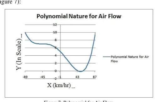
Air Flow:While selecting a better route through ocean, another criterion affecting the choice is Air Flow. Reports tell

that route with air flow 89 KM/H (in any direction, positive or

negative) should be avoided (thus given point 10 in the 10 point scale [5], to make it costlier). Routes with Air flow 45 KM/H in positive direction is a very good choice (so given 0 point to make it cheapest). However, routes with very minimal Air Flow is a moderate choice (given point 5 in the 10 point scale) and routes with Air Flow 45 KM/H in negative direction makes the situation worsen (thus given point 7 in the 10 point scale). Thus the following table is obtained:

Table 3:Air Flow

x(mt.) 89 45 0 -45 -89

y(scale) 10 0 5 7 10

Using the same procedure of Regression Analysis, discussed above, the following values of the unknowns is obtained:

Table 4: Values of the unknown variables used in (1) for Table 3

Co-efficient Values

c0 4.99994410760793

c1 −0.104490894607928

c2 −0.00121189124100473

c3 0.0000131916319554311

c4 2.3268915510016E−07 c5 −9.76631790679625E− 17

Thus the polynomial (equation) obtained for the parameter Air Flow is:

y =

4.99994410760793+(−0.104490894607928).x+(−0.001211891

24100473).x2+

(0.0000131916319554311).x3+(2.3268915510016E−07).x4+(−

9.76631790679625E− 17).x5

The graphical nature of the polynomial is as shown below Figure 7):

Figure 7: Polynomial for Air Flow

Water Current:Water current also plays a crucial role in ocean route selection. Path with current less than 0.4 m/s or more than 2.5 m/s should be avoided. Hence given 10 points, for making it costlier. Paths with current 1.3 m/s is best choice and awarded with 0 points to make it cheapest. Finally, path with current 0.85 m/s or 1.9 m/s is a moderate choice, with point 5 in 10 point scale. Thus the following table is reached: [6]

Table 5: Water Current

x(Mt./sec) 0.4 0.85 1.3 1.9 2.5

y(scale) 10 5 0 5 10

Using the procedure of Regression Analysis, discussed before, the following values of the unknowns is obtained:

Table 6: values of the unknown variables used in (1) for Table 5

Co-efficient Values

c0 3.14324

c1 40.77444

c2 -71.75304

c3 31.7

c4 0.63035

c5 -1.70556

Thus the polynomial (equation) obtained for the parameter Water Current is:

y = 3.14324 +( 40.77444).x+(-71.75304).x2+ (31.7).x3+(0.63035).x4+(-1.70556).x5

Thee graphical nature of the polynomial is as shown below (Figure. 8):

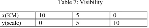
Visibility:During choosing a route through ocean, one also must consider the factor visibility. If it is even less than 1 KM, then the path should has to be avoided for sidetracking mishaps, hence given point 10 to make the route costlier. When visibility is near about 5 KM, makes the route a

moderate one choice; thus given weightage point 5 and finally

visibility 10 KM or more makes the route a best choice, so why weightage point 0 is associated then to make it cheapest. The following table illustrate the fact:

Table 7: Visibility

x(KM) 10 5 0

y(scale) 0 5 10

Without losing its generality, this data could be fit to a Linear Equation of the form:

 y = ax +b 

Putting the values, 3 simultaneous equations are obtained-

0=a.10+b (9)

5=a.5+b (10)

10=a.0+b (11)

Thus finally the equation takes the form as:

y = (-1)x +10

The graphical nature of the polynomial is as shown below (Figure 9):

Figure 9: Polynomial for Visibility

Possibility of presence of Sea Storm or Iceberg: Keeping mind the famous incident of “TITANIC”, any route with possibility of presence of Iceberg or Sea Storm is strongly being avoided. Thus here if no such possibility is there weightage 0 point is awarded and for such possibility, a very high sentinel value 99 is awarded, so that the route becomes so much costly, such that it would not come into crease even its distance factor is low. In other words, the path with such risks are strongly avoided even they are very short. Thus the following table is readily being achieved:

Table 8: Possibility of presence of Sea Storm or Iceberg

x (Is There any such Possibility?) 0 1

y(scale) 0 99

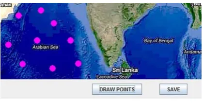
This procedure of finding OPTIMAL and SAFEST Route at first takes the Raster Map of any Sea/Ocean. It may be any scanned image/ Satellite image, which is not needed to digitize anyhow, making it less time consumed process. The reference cross points are marked by simply clicking onto them and parametric values like Depth of Water, Air Flow, Water Current, Visibility etc. are directly fed for each of this route-let. For the present method user-friendly GUI is there for accommodating these values.

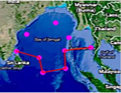
Finally, upon entering the Starting and Destination point of journey the technique performs Two-way-Tracking goal searching method and marks the Safeand Shortest Route by RED Line.

III. IMPLEMENTATION AND RESULTS

The results of enactment, design of GUI and all the required operations have been done using Net Beans IDE 8.0.2 (Java),

which is based on flat-file systems without using databases, hence have increased its portability.

The work begins with selection of a map (may be a scanned image or likewise) from any location of the computer. The start-up screen, Buttons for loading or adding new map selection of map, selecting new map are shown in the following

figures (Figure 10, Figure 11, Figure 12).

Figure 10: Start-up Window

Figure 11: Loading New Map

Next by clicking “DRAW POINTS” button, the reference cross-cross points are marked (Figure 13).

Figure 13: Digitizing Points

In the next step, the adjacencies of all the points to incorporate for analysis (i.e. Source, Destination and intermediate cross-points) along with distance between those

adjacent points and values of the influencing factors for those

paths are entered by clicking onto the “SET DISTANCE” (Figure 14) and “SET PARAMETER”(Figure 15) buttons respectively, after which the information being fed is saved by clicking “SAVE” button (Figure 16).

Figure 14: Setting Distance

Figure 15: Setting Parameters

Figure 16: Saving Data

Among the fed digitized point, any two can be selected as source and the destination points, which being fed by clicking

“SELECT SOURCE” (Figure 17) and “SELECT DISTANCE” (Figure 18) buttons respectively.

Figure 17: Selecting Source

Figure 18: Selecting Destination

At the final step, by clicking onto the “GENERATE PATH” button, the suggested Optimal Safest path from source to destination is displayed graphically by a red line (Figure 19 and 20).

Figure 20: Optimal Safest path

The above two figures depicts the fact that in different

season, due to change in various influencing factors, the path

between a pair of Source and Destination may also change.

IV. ANALYSIS AND COMPARISON

For analysis of the performance of the proposed TwT Method, the number of nodes varied from 2 to 1200 and the time was recorded. The following table (Table 9) summarizes the result.

Table 9: Performance of the TwT Method with increasing number of nodes

Number of Nodes Time Taken in

Milliseconds

10 5842

40 23725

100 47328

200 90883

300 132982

400 178943

500 223456

600 557223

700 869783

800 1572891

900 1934901

1000 2479541

1100 2815938

1200 3657892

Figure 21 shows the graphical representation of the data

reflected in Table 9

Figure 21: Performance of the TwT Method with increasing number of nodes

All the graph-based-Goal-search algorithms start there searching from Source node and traversing through the edges,

finally reaches at Destination node (or sometimes reverse).

Heuristic graph search algorithms have exponential time and space complexities as they store complete information of the path including the explored intermediate nodes. Hence many

applications involving heuristic search techniques to find

optimal solutions tend to be expensive. Despiteof these, the

researchers have strived to find optimal solution in best

possible time. Among many such existing algorithms, presently four algorithms- Generate – And – Test, Simple Hill – climbing, Steepest –Ascent Hill Climbing and BestFirstSearch[7], all of which are applied for finding the shortest path, have considered for comparison with the present technique Two-way-Tracking.

Generate – And - Test Method:

This algorithm first generates a path from the start state.

Then check whether it is a solution or not. If it a solution, then quit otherwise generate another path from start state. But there

is a limitation that there is no guarantee to find a solution.

Hence a comparison could be made as follows:

Table 10: Comparison between Generate – And – Test with Proposed

Algorithm

Generate – And – Test Proposed Technique (TwT) There is no guarantee to

find a solution.

There is guarantee to find a

solution.

Simple Hill Climbing Method:

The algorithm Hill climbing expands a particular node at the beginning of the search with the node which is considered as the source node. Every time it explores only the best possible node which is adjacent with present node. For that reason, this method does not undergo any complicated calculation and this phenomenon does not ensure the completeness of the produced results. The Hill climbing method does not give a desired result because this procedure may abort with a non-final state.

It can be noticed that, when algorithm is unable to reach to the destination node, then this state is denoted as failure state. This situation is occurred when the algorithm reached to a node from where no future exploration is allowable i.e. no new best node is available to expand. Thus the following comparison can easily be drawn:

Table 11: Comparison between Simple Hill Climbing with Proposed Algorithm

Simple Hill Climbing Proposed Technique (TwT)

May not find Complete

Solution i.e.it may not reach to the Goal node.

Definitely find Complete

Solution i.e. it must reach to the Goal node.

Steepest – Ascent Hill Climbing Method:

In this method, every node from present node is taken under consideration and among them the best one is to expand. In Simple hill climbing, the better successor comes first is selected and may neglect the best one. On the other hand, steepest ascent hill climbing method explore the better state maintaining

the steepest slope. This method finds the best successor node

among every available successor node without considering the

first best node as the desired one.

backtracking this procedure will be very much time absorbing.

As the method does not find the optimal solution i.e. does not

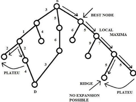
catch the goal state so the process after reaching a state from where there are no nodes are able to generate for further exploration. This will happen if the processing has meet with one of the following situations: (Figure22):

1. Selecting the node, better than its neighbors, may

overlook few better nodes. This defined as local maxima.

2. Selection of next best node between two same edge-weight successor nodes is seems to be difficult. This phenomenon is termed as plateau.

3. In a scenario where maintaining the local maximum drives to a particular node from where further exploration impossible, is termed as ridge.

Figure 22: Plateau, Ridge, Local Minima

Table 12: Comparison between Steepest – Ascent Hill Climbing Method with Proposed Algorithm

Steepest – Ascent Hill Climbing

ProposedTechnique (TwT) Method

May not find Complete

Solutionand also face problems due toRIDGE , PLEATUE and absence ofGLOBAL MINIMA.

Definitely find Complete

Solutionand also does no face problems dueto RIDGE , PLEATUE and

alwaysgive GLOBAL

MINIMA.

Best – First Method:

In graph search method Best first search [7] , a single node gets explored at each time simply by choosing minimum edge-weight. This minimum edge-weight is the outcome of estimating function which gives a demarcate of distance to the goal node.

Best first search may look like a combination of Breadth -First-Search and Depth--First-Search as it endures all the good notions of both the techniques. Depth-First-Search reaches goal without considering every node, in other hand, Breadth-First-Search method arrives at goal by exploring level by level. As Best-first search is a hybrid of these two it permits swapping between best paths. The Best-First Search method involves the properties of OR graph, in which vertex i∈ V(G) generated from j ∈ V(G) will maintain a PARENT LINK to j that will help to recover the path from Destination to Source. It needs two different lists for execution. The nodes with determined heuristic cost kept in list OPEN to explore in future. Already

traversed nodes are kept in CLOSE list. Hence, the following comparisons could be made with the proposed technique:

Table 13: Comparison between Best – First Method with Proposed Algorithm

Best – First Method Proposed Technique (TwT)

Does not find optimal

solution.

There is guarantee to find a

solution.

Comparison with AND-OR Graph:

Although the present TwT method has used some properties of ANDOR-Graph, but to increase the efficiency of the present method several measures has incorporated to reduce the number of Backtracking. Hence the following comparison can be made:

Table 14: Comparison between AND-OR Graph with Proposed Algorithm

AND-OR Graph Proposed Technique (TwT)

Several Backtracking involves,making it more time consuming.

Comparatively a large amount of Backtracking is reduced.

Comparison with Chandel’s Bi-Directional Search [7]:

Chandel et.al.introduced a new graph search technique, known as Bidirectional Search which traverses the graph in both the direction, just like the present method. But the problem with bidirectional search is that it has not incorporated any method for reducing times due to backtracking or likewise; causing it to take a lot of execution time. Moreover, this technique doesn’t always work properly; because if the graph is

more connected then it is less beneficial in case of applying

bidirectional search. But in case of TwT; two way search has been used to decrease execution time and it does not get restricted for any type of graphs.

Comparison with Dijkstra’s Method:

For some graph searching problems, TwT reaches the Goal node faster (using fewer numbers of iterations) than using Dijkstra’s Method. The following graph (Figure 23) presents one such scenario:

Figure 23: Graph for comparison with Dijkstra’s Method

Here Source node is S and Destination node is D. Here starting from S, Dijkstra’s Algorithm will touch the nodes N,

M, O respectively in the first three iterations. Searching

successful search. Thus here TwT completes searching just after second iteration, much before than that of Dijkstra’s method. This has been elaborated in the following table(Table):

Table 15: Moves made in the Graph shown in Figure 23

Number of Iteration

Dijkstra’s Algorithm

Proposed Algorithm Triggered

fromsource S

Triggered fromdestination D

First N N Q

Second M M S (Successful

& Terminates)

Third O S -

The output produced by the Goal Searching Algorithm can

be considered as Boolean, either Success (able to find the Goal node) or Failure (Unable to find the Goal node). Some

algorithms might get stuck in an infinite loop and never return

an output.

For comparing different Graph-based-Goal-Searching Algorithms, the following metrics are useful:

Completeness: This depicts the fact that whether the

algorithm guaranteed to find a solution when there is one. Obviously, algorithms having Completeness property are of prime interest, both for theoretical and practical applications.

Optimality: This points to the fact that whether the

algorithm is able to find an Optimal Solution or not. Surely,

algorithms able to find optimal solutions are of particular

interest than others.

Time Complexity: This is related to the execution time of the algorithm. Generally, the order of search time complexity of the algorithm is expressed as a function.

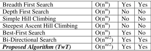
The following table reflects a concise comparison among

various Graph-based-Goal-Searching Algorithms, in addition to the present technique.

Table 16: Comparison among various Graph-based-Goal-Searching Algorithms

Breadth First Search O(nm) Yes Yes

Depth First Search O(nm) No No

Simple Hill Climbing O(nm) No No

Steepest Ascent Hill Climbing O(nm) No No

Best-First Search O(nm) Yes No

Bi-Directional Search O(nm/2) Yes Yes Proposed Algorithm (TwT) O(nm/2) Yes Yes

Where,

m = depth of solution with in search tree n = branching factor of search tree

V. CONCLUSION

The present technique is a kind of goal searching algorithm in a weighted graph, where the Optimal and safest route between Source and Destination has been found. So this technique can be applied in a number of challenging fields in

GIS. Presently one such application area, finding shortest as

well as safest route through ocean has outlined.

The proposed work is in a way to stretch its helping hand for minimizing these heart breaking incidents. It foretells the captain about the safest route for propelling. The graphical outcome makes it very much understandable to anybody.

This technique cannot only be applied for the avoidance of road accidents and plane crashes due to selection of wrong route or decrepit road for traveling, by simply changing the

influencing factors; but could play as a guide while solving

Land Acquisition problem. While acquiring land for the purpose of new constructions, like Highway or Rail-route deserted/ low fertile lands should be preferred but this should

not enlarge the route.Thus finally this is also a goal reaching

problem through cheapest (in terms of factors considered) route.

VI. ACKNOWLEDGMENT

The authors are thankful to Department of Computer Science, BarrackporeRastraguruSurendranath College, Kolkata-700 120,W.B., India for providing all the infrastructural support to carry out the intended work.

VII. REFERENCES

[1] Elaine Rich, Kevin Knight, Shivashankar B Nair, ARTIFICIAL INTELLIGENCE, PHI, Third Edition

[2] Isra’a Abdul-Ameer Abdul-Jabbar, Suhad M. Kadhum, Adaptive Backtracking Search Strategy to Find Optimal Path for Artificial Intelligence Purposes, Computer Engineering and Intelligent Systems ,ISSN 2222-1719 (Paper) ISSN 2222-2863 (Online),Vol.5, No.2, 2014

[3] RINA DECHTER ,JUDEA PEARL ,GENERALIZED BEST FIRST SEARCH STRATEGY AND OPTIMALITY OF A*,Report No.CSD – 840068 , December 1984

[4] Dr. S A MOLLAH , NUMERICAL ANALYSIS and COMPUTATIONAL PROCEDURES , PHI, Fourth Edition

[5] www.baynews9.com/content/news/baynews9/weather/hurricane center/wind- speeds.html

[6] hypertextbook.com/facts/2002/EugeneStatnikov.shtml