!
"!"
# $ $"
%
&
''' (
Performance Evaluation of Classifier Models Using Resampling Techniques
Swarnalatha Purushotham*
School of Computing Science and Engineering VIT University,
Vellore,India [email protected]
Dr.S. Prabu
School of Computing Science and Engineering VIT University,
Vellore,India [email protected]
Abstract: One of the important datamining function is prediction. Many predictive models can be built for the data. The data may be continous, categorical or combination of both. For either of the above type of data many similar predictive models are available. So its highly important to choose the possible best accurate predictive model for the user data . For this the models are evaluated using resampling techniques. The evaluated models gives statistical results respectively. These statistical results are analysed and compared .The appropriate model that gives maximum accuracy for the user data is used to do predictions for further data of same type. The predictions thus made by the best model can be visualized. They form the decision reports for the user data.
Keywords: Dataset, Resampling Technique, Cross validation, Accuracy, Class label, Training data, Test data, Model induction, Model deduction.
I. INTRODUCTION
In today’s Competitive Corporate world, Research field and Medicine it is highly necessary to make predictions for the huge available data in order to classify them into different categories. These data are taken in the form of dataset which is a collection of data in rows and columns, where each row is a set of data or instance. Prediction identifies to which class or value each instance belong to. The prediction is a single dependent value which is either a categorical or a continuous one for a single set of independent data or instance. Classification and Regression models are needed respectively to do such prediction. These models are built on a sample population and then used to do the prediction in the target population of the same domain. But again several classification and regression models are available. So it’s very important for us to choose the appropriate Predictive model among several similar models, such that it produces the reliable predictions for the supplied data. For this predictive models are first constructed on a dataset and evaluated using resampling techniques which gives quantifiable statistical results. Finally Statistical Analysis is done to obtain the possible best model. In this paper Classification models are taken into evaluation and analysis. These models does the categorical or nominal prediction only.
Wherever Times is specified, Times Roman or Times New Roman may be used. If neither is available on your word processor, please use the font closest in appearance to Times. Avoid using bit-mapped fonts if possible. True-Type 1 or Open Type fonts are preferred. Please embed symbol fonts, as well, for math, etc.
II. METHODOLOGIES
Machine learning is the core technique in modelling. The goal of machine learning, is to build computer systems that can adapt and learn from their experience. Thus bringing in the concept of artificial intelligence [5]. This
technique is used in model induction or model training. A classifier is a function that maps an unlabelled instance to a label using internal data structures. An inducer or induction algorithm builds a classifier from a given dataset. In this paper we are not interested in the specific method for inducing classifiers, but assume access to a dataset and an inducer of interest.
Supervised learning is a machine learning technique for learning a function from training data. The training data consist of pairs of input objects (typically vectors), and desired outputs. The output of the function can be a continuous value (called regression), or can predict a class label of the input object (called classification). The task of the supervised learner is to predict the value of the function for any valid input object after having seen a number of training examples. This is model deduction.
For evaluation resampling techniques [2] such as cross validation, bootstrap and holdout method are available. Resampling refers to repeated random sub sampling of data from the original dataset into training and test data. In our evaluation we use cross validation to split the given data into training data and test data which are independent of each other. After splitting, build the model with training data and evaluate with the test set to get the accuracy rate and various supporting statistical results, which is a helpful in comparing models and find the best classifier for the data.
III.EVALUATION
design as if these test cases didn't exist. Having large numbers of hidden test cases is atypical of most real-world situations. Normally, one has a given set of samples, and one must estimate the true error rate of the classifier. Unless we have a huge number of samples, in a real-world situation, large numbers of cases will not be available for hiding. Setting aside cases for pure testing will reduce the number of cases for training. More the training data the performance of the classifier is better and also more the no of test data the estimation can be better.
Training and testing the data mining model requires the data to be split into at least two groups. If you don’t use different training and test data, the accuracy of the model will be overestimated[6]. The resampling technique is applied to create mutually exclusive repeated training and test partitions. The particular resampling methods that should be used depends on the number of available samples. Here are the guidelines:
A. For sample sizes greater than 100, use cross-validation. Either stratified l0-fold cross-validation or leaving-one-out is acceptable.
B. For samples sizes less than 100, use leaving-one-out. 10-fold is far less expensive computationally than leaving-one-out and can be used with confidence for samples numbering in the hundreds. This technique can be used as a standard estimation technique as various theoretical proof suggest that this method has low variance and better reliable accuracy for dataset of all sizes and it is unbiased.
Data is split into k subsets of equal size. The instances for each subset or fold are randomly selected. Each subset in turn is used for testing and the remainder for training a particular model. This training and testing is done for k times such that each subset is used once as the test set. The disadvantage of this method is that the training algorithm has to be rerun from scratch k times, which means it takes k times as much computation to make an evaluation. Thus we get k error estimates. In stratified tenfold cross validation, each fold is stratified so that they contain approximately the same proportion of class labels as the original dataset. By this variance among the estimates are reduced and the average error estimate is reliable. The test set is a group of labelled instances that were not used in the training process. So when the test set is deduced on a trained model, the model classifies the instances (model deduction). These classified instances are compared with actual labels and from this we deduce the accuracy and several misclassification details. The misclassification details are mentioned in detail in later part of the paper.
Accuracy of a classifier is defined as the number of correctly classified instances divided by total no of test instances taken. Error rate is calculated as (1- accuracy rate). Significance Tests
Given a classier and an estimate of its error, the true error might be substantially higher or lower than the estimate. When the sampling distribution is skewed (asymmetric), as is usually the case for error rates, a correctly defined confidence interval is more informative than the standard deviation. Another way is to specify a confidence interval, a region which contains the relatively plausible values of the true error. One way to do this is to give the standard deviation of the estimate's sampling distribution. Statistical Inference is obtained from the
evaluation methods. The topics dealt with in this module, a different aspect of statistical inference and hypothesis testing- “using sample information to answer questions about the population and the Inferred classifier”.
One such question is whether the classifier correctly predicts the classes. The various methods for estimating error can be thought of as alternative methods for assessing the truth of the hypothesis that the classifier's predictions are correct. If we knew or assumed that the population data were free of any measurement, observation, or labelling errors, then the occurrence of a single prediction error would serve to refute the hypothesis. If we know or can reasonably assume that the population data are imperfect, as is typically the case, then a single prediction error is not sufficient to refute the hypothesis (it could be that the prediction is right and the data are wrong). In the latter circumstance, we must accept or reject the hypothesis based on an inference regarding the strength of the contradictory evidence relative to the reliability of our data.
Another hypothesis that we frequently wish to test is that the true errors of two alternative classifiers are different, i.e., that one classifier predicts more accurately than the other. This question is more conveniently posed as a test of the null hypothesis that the true errors are equal. Again, typically we must accept or reject the hypothesis based on an inference regarding the strength of the contradictory evidence relative to the reliability of our data.
Thus, the ability to answer the following two questions is particularly important:
(1) How reliable is our estimated error, e.g., within what interval is the true error to be found with a 95% (or 99%) likelihood?
(2) Given another classifier having a different estimated error, how confident can we be that its true error is different from that of the first classifier?
IV. CONFIDENCE INTERVAL
With the estimated accuracy rate we can expect that the future true performance of this classifier will be around close to the estimated accuracy rate. But how far it is close? Within 5% TO 10%. So we have to perform various statistical analyses [3] on the results to get the confidence internal of the estimated accuracy rate. For this we use the Bernoulli trial, binomial distribution of Bernoulli trial and standard normal deviation method to find the confidence interval. With the confidence interval given for a particular classifier, the future predictions on the same model can deviate within these intervals, so that we can believe the predictions are mostly accurate.
Thus the confidence interval is obtained.
V. MODEL COMPARISON
When comparing two learning schemes by comparing the average error rate over several cross validations, we are effectively trying to determine whether the mean of set of samples- samples of cross validation estimate that is significantly greater than or significantly less than the mean of the other. This job for a statistical device known as the t test, or Student’s t test [7]. Because the same cross-validation split can be used for both methods to obtain a matched pair of results, one for each scheme, giving a set of pairs for different Cross validation splits, a more sensitive version of the t- test known as paired t – test can be used. The following procedural steps explains the required.
A. Procedural Steps of Model Comparison
The individual samples are taken from the set of all possible cross-validation estimates. We can use a paired t-test because the individual samples are paired.
[a] The same CV is applied twice. Let x1, x2, …, x k and y1, y2, …, yk be the 2k samples for a k-fold CV. The distribution of the means are as follows,
[b] Let mx and my be the means of the respective samples [c] If there are enough samples, the mean of a set of
independent samples is normally distributed.
[d] The estimated variances of the means are x^2/k and y ^2/k. . If µx and µy are the true means then mx - µx/ x^2/k , my - µy / y ^2/k , are approximately normally distributed with 0 mean and unit variance. [e] Let md=mx-my, The difference of the means (md) also
has a
[f] Student’s distribution with k-1 degrees of freedom [g] Let d ^2 be the variance of the difference.
[h] The standardized version of md is called t-statistic t= md/ ( d^2)/k .
[i] Fix a significance level . Look up the value for z that corresponds to /2.
[j] If t -z or t z then the difference is significant
[k] I.e. the null hypothesis can be rejected. There is significantly some difference between the accuracy of two predictive models.
[l] Else, null hypothesis is accepted. There is no real difference between the two predictive models.
B. Model Saelection
A classic metric for reporting performance of machine learning algorithms is predictive accuracy. Accuracy reflects the overall correctness of the classifier and the overall error rate is (1 - accuracy). If both types of errors, i.e., false positives and false negatives, are not treated equally, a more detailed breakdown of the other error rates becomes necessary.
Accuracy has many disadvantages as a measure. These are its basic shortcomings:
[a] It ignores differences between error types
[b] It is strongly dependent on the class distribution (prevalence) in the dataset rather than the characteristics of examples.
Apart from accuracy, the misclassification cost should also be considered because a patient with a disease symptom predictive negative is of more risk compared to a patient with no such symptoms but predicted positive. Performance
of a learning scheme includes many such statistics such as precision, recall (sensitivity), F-measure, true positive rate, false positive rate etc. Even these parameters are used to compare classifiers. This is considered to be second supervised learning. Thus a model comparison chart is generated as follows
The accuracy rate and its confidence interval are taken into consideration. The interval should not be very large as it suggests that the true accuracy rate can deviate widely. The following figure is confusion matrix showing the deviation of predictions from the actual class.
Figure 1: Confusion Matrix
From the confusion matrix other statistics such as true positive rate or sensitivity or recall (the accuracy among positive instances and specificity among negative.) and true negative rate is calculated.
In the evaluation of information retrieval systems, the most widely used performance measures are recall and precision.
Based on these misclassification costs and significance tests made the best appropriate model is selected.
C. Model Deduction
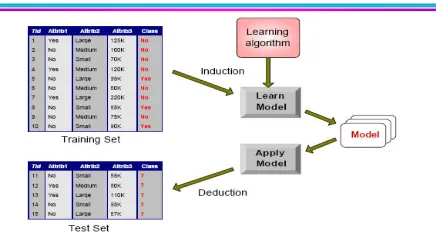
The best model from the above evaluation method is taken and it is supplied with a new test file whose instance class labels has to be predicted. The best model gives the appropriate prediction for the new data of the same domain, with the attribute type, name being the same with the original data on which the model was built. The predicted class value for each instance is displayed for the given test file. Fig 2 explains the model induction and deduction..
VI. EXPERIMENTAL RESULTS
The dataset is taken as Comma Separated file format or Attribute Relation file format(*.arff). The same dataset is used to build different classifier models. The trained models are evaluated on the same resampling technique called stratified tenfold Cross Validation. The dataset used in our experiment is Iris dataset [4] which has 150 instances having three class labels (setosa/versicolor/virginica), each distributed in equal proportion. Three classifier models are taken into consideration namely Decision Stump, BF tree and J48. Their respective inducer algorithms are used to build the classifiers. All these models can predict nominal data. Cross validating thses models produces the following output,
A. Stratified cross validated estimates such as no of correctly and incorrectly classified instances, average accuracy rate, kappa static.
B. Detailed accuracy by each class such as recall, precision, false positive rate, F-measure.
C. Confusion matrix showing misclassification details as shown below for the iris dataset classification.
a b c <-- classified as 50 0 0 | a = Iris-setosa 0 46 4 | b = Iris-versicolor 0 5 45 | c = Iris-virginica
The following table shows comparitative statistical details of three classifier models. The recall, precision and false positive rate are given for the three class labels – setosa, versicolour, virginica respectively under each misclassification.
Table 1: Statistical Comparison Chart For Three Models
Model
Accuracy rate(Confidence Interval)
Recall Precision False positive Rate
J48 0.98(0.94– 0.98) 0.98 0.94 0.96
1.0 0.94 0.96
0.0 0.03 0.03
Decision Stump
0.67(0.62-0.72) 1.0 1.0 0.0
1.0 0.5 0.0
0.0 0.5 0.0
BF Tree 0.94(0.92 – 0.97) 1.0 0.93 o.91
1.0 0.91 0.92
0.0 0.06 0.05
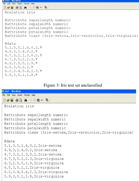
After all these evaluation, the best predictive model is selected according to the interest of the application in which the model is going to be applied. In our experiment results J48 is chosen as the appropriate model because of higher accuracy, narrow confidence interval for the true accuracy rate, higher recall and deduced for a new test file whose class labels are to be predicted. Fig 3 shows unclassified instances of iris test dataset and fig 4 shows the classified iris set after model deduction.
Figure 3: Iris test set unclassified
Figure 4: Iris test set classified by J48 model
VII. CONCLUSION
By this evaluation system the classifiers are compared statistically by significance tests [4] and provide an improved comparison schemes which gives more insight into the true error rate and misclassification costs. This provides a better evaluation methodology to choose the appropriate predictive model for the data and can make possible reliable predictions.
VIII. ACKNOWLEDGMENT
Swarnalatha Purushotham, member of IACSIT, Vellore, 04.11.77. M.Tech (CSE), VIT, Vellore, Pursuing Ph.D (Intelligent Systems). Assistant Professor (Sr), in the school of computing sciences and engineering, VIT University, at Vellore, India, has published more than 15 papers and guided many students of UG and PG so far. She is having 10 years of teachin experiences. She is associated with CSI, ACM, IACSIT, IEEE(WIE). Her current research interest includes Image Processing, Neural Networks, Pattern Recognition, Remote Sensing.
IX. REFERENCES
[1] Statistical Tests for Comparing Supervised Classification Learning Algorithms, Thomas G. Dietterich, [email protected], Department of Computer Science , Oregon State University, Corvallis, OR 97331, January 27,1997.
[2] Ron Kohavi,”A Study of Cross-Validation and Bootstrap for Accuracy Estimation and Model Selection”, Computer Science Department Stanford University, Stanford, CA 94305,ronnykGCS Stanford EDU,kohavI 1137-1143, h t t p / / r o b o t i c s Stanford edu/"ronnyk.
[3] Chris Drummond,”Machine Learning as an Experimental Science (Revisited) ”, Institute for Information Technology, National Research Council Canada, Ottawa, Ontario, Canada, K1A 0R6, [email protected].
[4] Ian H. Witten, Eibe Frank, Len Trigg, Mark Hall, Geoffrey Holmes, and Sally Jo Cunningham,” Weka: Practical Machine Learning Tools and Techniques with
Java Implementations”, Department of Computer Science, University of Waikato, New Zealand.
[5] D. Jensen. Labeling space: A tool for thinking about significance esting in knowledge discovery. Office of Technology Assessment, U.S. Congress, 1995.
[6] D. Wolpert. On the connection between insample testing and generalization error. Complex Systems, survey page nos.6:47–94, 1992.
[7] Olivier Gascuel & Gilles Caraux, “Statistical Significance in Inductive Learning”, Departemendt '/nformatiqueF ondamentaleL, IRMM 860 rue de Saint Priest, 34090 Montpellier, France, ascuel@crimfr European Conference on AI, Vienne, Wiley, pp. 435-439, 1992.
[8] P. M. Murphy. UCI repository of machine learning databases – a machinereadable data repository. Maintained at the Department of Information and Computer Science, University of California, Irvine.Anonymous FTP from ics.uci.edu in the directory pub/machinelearningdatabases,1995.