A Procedure for Rapid Collection, Processing, and Analysis of Line Intercept Data.

(1)

and Analysis of Line Intercept Data1

GEORGE M. VAN DYNE

Asst. Prof., Range Nutrition and Measurements, Animal Industry and Range Management Department, Montana State College, Bozesman, Montana.

The line intercept technique,

essentially that developed by

Canfield (1941)) has been a use-

ful measurement procedure in

range investigations. Some of the criticisms of this technique have qnvolved the subjectivity of the method, the time which it takes to locate and read line transects, and the difficulty in replacing line transects in the original po-

sitions for rereading. Many of

these objections may be over-

come by application of the technique for locating study units as

explained by Van Dyne (1959)

and by the use of the mechanical

range measurement device de-

scribed by Fisser and Van Dyne (1960). Line transects may be installed and relocated rapidly, and highly objective repeatable readings may be made by using these techniques. The se techniques have been used success- fully during the last two field seasons. Use of these procedures has resulted in the collection of

an immense volume of data

which made necessary adequate

Vegetation of the study area These investigations were con-

ducted on a southcentral Mon-

tana foothill range containing a

1 No endorsement of any particular make of electronic equipment is in- tended although these data were processed entirely by IBM ma- chines in the Montana State Col- lege Statistical Laboratory. Othe? types of electronic equipment could be used with equal efficiency. Jour- nal paper number 487, Mont. Agric. Expt. Sta.

Acknowledgement is extended to the Statistical Laboratory and Herb Fisser, former graduate student, for their interest and aid in these in- vestigations.

compilation, summarization, and

analyses procedures.

mixture of grasses and forbs

with a few scattered shrubs. The total basal density of all vegetation as determined by line inter-

cept techniques in the study

area averaged approximately 30

percent. Herbage production in

the pastures in which these techniques have been applied aver-

aged approximately 500 to 750

pounds per acre. The dominant species were blue grama grass

(Bouteloua gracilis), bluebunch

wheatgrass (Agropyron spic-

atum), needle-and-thread grass

(Stipa comata), western wheat-

grass (Agropyron smithii), june- grass (Koeleria cristata), needle- leaf sedge ( Car ex eleocharis),

blazing star (Liatrus punctata),

Hood’s phlox (Phlox hoodii),

scarlet globemallow (Sphaeral-

(Lupinus serecius).

Field procedures

Two techniques, manual re-

cording and a portable tape recorder (Figure 1) , were used in the field to record data. Taped data were later transcribed onto the special forms by non-scientific personnel. Most of the data were

tape

recorded to better util- ize the time of trained personnel in the field work. Approximately

6 to 8 minutes of recording time were necessary per transect as compared to 15 to 25 minutes of reading time. In the field, the

tape recorder was powered by

either a 12-volt or a llO-volt elec- trical system.

The forms on which the data were recorded have a location at the top of the page for control information regarding the study, such as project number, location, treatment, and replication. The

intercepts were verbally re-

corded by reporting first a type code; second, the name symbol of a species or other intercept; and third, the point where that particular intercept began. Fig-

(2)

248 VAN DYNE

TRANSECT DATA FIELD SHEET

Replication 2

FIGURE 2. The front of the form used for recording data. This form was used for re- :ording directly in the field and for recording transcribed data which were dictated in the field.

ure 2 shows a completed form. Intercept position numbers are a part of the field forms and are used in studies of species inter- relationships.

Coding of intercept data Each species was given a type code number, depending upon its growth form, to aid in summarization of data by growth form for tabular presentation or for

statistical analyses. The type

code numbers from 10 through 19 were reserved for vegetation intercepts, the numbers from 20 through 29 for intercepts on animal material, and the numbers 30 through 39 for intercepts on mineral materials. This organi- zation of type codes has allowed

for rapid machine summariza-

tion and analyses for these ma-

jor groupings. Within each of

the type groups there were vari-

ous sub-groupings as shown in

the following example for vegetation:

Type lo-perennial grasses

Type 1 l-annual grasses

Type 12-sedges, rushes, and

grass-like

Type 13-annual forbs

Type 14-biennial forbs

Type 15-perennial forbs

Type 16-half-shrubs Type 17-shrubs Type 18-trees

Type 19-miscellaneous vege-

tation

The coded plant names were composed of six-letter symbols. The first four letters of this symbol were a standard species symbol involving the first two letters of the generic name and the first two letters of the species name. The fifth letter position in this symbol was normally left blank, but was used in a few cases for control of duplication

of symbols. For example, 10

STCO is the coding for Stipa comata, as well as for Stipa colum-

biana, both being perennial

grasses. In this case, a “2” was

recorded after the symbol for

St ip a columbiana indicating it

was the second most common perennial grass species with the symbol 10 STCO. Two species of different growth forms, in some instances, had the same symbol such as CHVI for Chrysotham-

nus vicidiflorus and Chrysopsis

villosa. In this example, how-

ever, since the two species are of a different growth form, there is no need for a duplicate control number as they can be separated by the type code. The sixth pos- sible letter in the name was used to record supplementary inf or-

mation regarding the hit. For

example, a “D” was recorded in this column for dead material of the particular species involved, an “0” for an overstory hit, an “S” for a seedling. Upper case letters were used throughout to minimize confusion because the IBM equipment printed only upper case letters.

(3)

a 3 SF 2 3 SF

3, e 1 1 e 3 1 e

33 ” 1.9 1ss .36

FIGURE 3. A listing of the lengths and position of intercepts of the data presented on the form in Figure 2. Each line of data represents a card. Lengths are presented in hundredths of feet.

were used to record hits on fecal material of rodents, cattle, sheep,

and horses, respectively. Type

codes 31, 32, and 33 were used to code the mineral hits of bare ground (B) , rock (R>.03’ diam-

eter) , and erosion pavement (.Ol’

<P<.O3’), respectively. Appro- priate one- or two-letter abbrevi- ated name symbols were used to record all animal and mineral intercepts and litter.

Intercepts were recorded in

the nearest 0.01 foot along the five-foot transect lines. A useful

check in recording data is appar- ent in that each successive inter-

cept must begin on a higher

number than did the preceding one. A “500” was entered as the

last “beginning of intercept”

without any species name for

purposes of machine calculation of the length of intercepts.

Compilation procedures After the transect data field sheets were briefly reviewed and obvious errors corrected, the material was taken to the Statistical

Laboratory for key-punching

(IBM 026). Key-punching was a

rapid process, approximately 500 to 600 cards per hour, due to the nature of the special field form used in collecting the data. After the data were key-punched, the cards were verified.

A process involving the reading of two successive cards in different card-reading cycles in

the tabulator (IBM 402) was

used in determining the length of each intercept. The end of a given intercept is determined by the beginning of the following intercept. In this procedure, the first card was run into the tabulator and at the second reading position its intercept was compared to that of the following

card at the third reading position. (A wiring diagram for the IBM 402 for this procedure is available on request.) All control data, the intercept number, the type and name, the beginning of the intercept, the end of the intercept, and the length of the intercept were punched on a separate card on the repro- ducer (IBM 514).

The cards were then sorted alphabetically by species within plant groups and a complete list of the data was made for each transect. Figure 3 shows a list of the data from the transect shown on the form in Figure 2. Figure 3 and the following two figures are IBM tabulator sheets. The columns and/or rows have been labeled to indicate the type of data in each. By checking the list of intercepts it was easily

noticed when a card came

through with a “negative intercept.” That is, where an error was made in recording data and

the end of intercept was a

smaller number than the beginning of the intercept. Only 12 of these negative intercepts oc-

curred in approximately 14,000

cards of line intercept data collected on one project in the 1959 field season. All of these errors

2 c21 1 10 BOCR 2 c21 1 10 CAM0 2 c21 1 10 KOCR 2 c21 1 10 STCO

2 c21 1 12 CAEL

011 007

004 004 TOTAL OF LENGTH

004 002 AND NUMBER OF

002 00 1 INTERCEPTS

21 014 FOR:

003 003 -TYPE IO

3 003

2 c21 1 15 OXSE -TYPE 12

003 00 1 2 c21 1 15 PHI-IO 00 1 00 1

4 002

2 c21 1 19 L 138 015 -TYPE 15

2 c21 1 IS SEDE 145 U16 2 C21 1 19 SEDE D 106 011

391 042

7 C21 1 23 SF 009 002 -TYPE 19

9 002

2 C21 1 31 8 028 003 - TYPE 23

z-6 -2 -TYPE 31 2 C21 1 32 P 028 002

28

2 c21 1 33 R 0 16 00 1 002 - TYPE 32 16 001 - TYPE 33

so0 +s

TOTAL OF ALL INTERCEPTS LENGTHS AND NUMBERS

(4)

250 VAN DYNE

Iv ₁

1 R 3 44878 2243900

7 A 2 17053 R52650

3 AR 4 2731 1 682775

4 e 2 52‘3)08 2645400

5 AB 4 57Je 1 1439525

6 BR 4 34dO6 870150

7 A6R 6 37246 465575

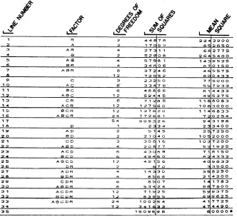
FIGURE 5. A listing of the results of the analysis of variance program for basal cover of blue grama. In this analysis N = 216.

were due to obvious recording or

punching mistakes and were eas-

ily corrected.

Summarizing for species and plant groups

Sorting the cards of data into

order of plant names (alphabet-

ically) within type codes for each

transect was accomplished at a

rate of approximately 600 cards

per minute using the IBM 082

sorter. On any one transect a

given species may have occurred

several times, thus several cards

contained data for that species

on the line. These data were

summarized on the tabulator so

that a minor total was made of

the intercepts on all cards of

each species occurring on the

transect, an intermediate total

was made of all the intercepts

of the species of a given type

code, and a major total was made

of all the intercepts on the tran-

sect. The latter total, necessarily

500, provided a means for a sim-

ple check. In addition to printing

and punching the total length of

intercept for each species, type,

and transect, the total number of

times the intercept occurred was

punched in the card.

The data from the transect

presented on the field form in

Figure 2 and listed by species

in Figure 3 are shown in sum-

marized form in Figure 4. The

list shown in Figure 4 provides

a means of rapidly assessing the

importance of different species

over the experimental area and

an excellent opportunity for a

last visual check before statisti-

cal analyses.

Statistical analyses

These data were collected from

a project which was designed as

a three square factorial with

three replications, four plots per

treatment, and two transects per

plot. A standard program deck

has been punched for this analy-

sis, so that the necessary compu-

tations may be conducted easily

with the IBM 650 electronic com-

puter. (This is North Carolina

State program 6.4.001.1 for the

IBM 650.) It took approximately

6 to 8 minutes to conduct an

analysis of variance on a given

variable. The data obtained from

this analysis includes all the in-

formation that is necessary for

the analysis of variance table ex-

cept for “F” determinations

which can be easily computed

with a hand calculator. Figure

5 shows the sums of squares, de-

grees of freedom,

and mean

squares attributable to the vari-

ous factors in an analysis of vari-

ance of the basal cover of blue

grama grass. Analysis of vari-

ance may be easily conducted for

an individual species or for a

group of species such as peren-

nial grasses, all mineral inter-

cepts, or all miscellaneous vege-

tation.

The necessary mean squares

were summed on a desk calcu-

lator and the F values were de-

termined by use of a desk calcu-

lator. The mean values for the

factors desired are easily com-

puted on the IBM 650 electronic

computer.

Evaluation of procedures

The procedures described for

collection, processing, and analy-

sis of line intercept transect data

are sufficiently flexible

to be

used in recording other types of

measurement data. Similar pro-

cedures have been used success-

fully in processing and analyzing

weight data, height data, and

counts of plants.

Additional

range plant characteristics may

be coded for grouping in anal-

yses such as grazing response,

season of growth, and height

class.

Coding of range plant names

by alphabetic symbols was very

useful in the field work due to

the flexibility of the system.

Coded range plant names were

also conveniently

read on

(5)

*

mately twice the time as sorting

on numerical information.

The use of electronic data

processing equipment is r el a -

tively new to many range re-

searchers

and administrators,

and considerable time must be

spent in securing an understand-

ing of the equipment and pro-

cedures.

These procedures have pro-

vided for the collection of a max-

imum amount of data during a

short field season. The data are

collected in such a manner that

non-scientific personnel

may

transpose them to standard

forms. The electronic data proc-

essing equipment used prior to

statistical analyses is very eco-

nomical compared to hand tabu-

lation. The statistical analyses

are very rapid compared to the

use of and checking by desk cal-

culators. The accuracy of the

data, completeness of analyses,

and earliness of availability for

publication purposes all favor

these techniques.

LITERATURE CITED CANFIELD, R. H. 1941. Application of

the line intercept method in sam- pling range vegetation. Jour For. 34: 388-394.

FISSER, H. G. AND G. M. VAN DYNE. 1960. A mechanical device for repeatable range measurements. Jour. Range Mangt. 13:40-42. VAN DYNE, G. M. 1959. A method for

random location of study units in

range investigations. Jour. Range

Mangt. 13: 152-153.

Determining Correct Stocking

Rate on Range Land1

L. A. STODDART

Professor of Range Management, Utah State University

Range technicians have been

recipients of considerable abuse

and criticism because of their

seeming inability to correctly

diagnose the grazing capacity of

the range. Actually, the manage-

ment and conservation of land is

one of the most essential and

noble of all the professions of

man. The land is our wealth and

our future. Care of this basic

resource is vital not only to the

agriculturist as a direct user but

to every American.

Land problems seem particu-

larly critical on western ranges,

where shallow, rocky, and salty

soils combine with aridity to re-

duce vegetation production to a

minimum and where steep and

rugged topography

encourage

rapid erosion. This delicate bal-

ance with which nature has en-

dowed so much of the range land

makes proper use and good man-

agement paramount in impor-

tance.

More than half of these ranges,

and certainly the most critical

1A paper delivered before a confer- ence of federal range technicians and stockmen held in Salt Lake City, Utah, February 16, 1960, to discuss methods of determining capacity of rangelands.