Search | Preprints

(1)

1

Warning Credit Risk for Vietnamese Commercial Banks - Case Study: Corporate Customer

Assoc. Prof, PhD. Nguyen Van Huan; Dr. Nguyen Thi Hang; Mr. Do Nang Thang Faculty of Economic Information System - Information and Communication

Technology Thai Nguyen University

Abstract: Stemming from the urgency of the actual situation, commercial banks need an effective credit risk management tool to limit risks. The authors went to survey, study and propose a set of factors affecting the ability of debt repayment of individual customers and conducting surveys. The topic uses data sets including 240 observation samples. Using the SPSS software to clean data and run the model based on Maddala's Binary logistics regression published in 1984 to find out the impact of each individual element of customers affecting their ability to repay such debts. Come on. The authors also specify the order of influence of each factor determining the ability to repay individual customers, thereby helping bank managers have a better visual view to make decisions for borrowing accurately, limiting risks.

Keywords: warning model, credit risk, logistics model

1. Introduction

Credit risk management is a very important activity it has received interest of every banks, currently there are many research projects on the world related to this research problem, of which typical is the Merton Model (1974) has an enlightening role in field of credit risk management, this model defines debt repayment ability of the company based on the calculation company's asset value at some time and compared with the company's debt with the assumption that the company only has a debt and has to pay at a single time, this is the limitation of the Merton model because the debt structure of the companies is very complex now. To overcome the limitations of the grading model depends a lot on the qualitative data, Altman (1977) has produced the Z score model. Model Z score calculates the customer's repayment capability base on historical data of factors affect to customer's repayment ability. The Z-score model used a multi-factor difference analysis method to quantify the probability of default of borrowers overcoming the disadvantages of the qualitative model, thus contributing positively to controlling Credit risks at commercial banks. However, this model is highly dependent on how to classify risky and risk-free borrowers. On the other hand, the model requires a fully updated information system of all customers. This requirement is very difficult to

(2)

2

implement in an inadequate market economy. The CreditMetrics model, introduced by JP Morgan in 1997, is a model commonly used in practice. This model can be viewed as derived from the Merton model, however there is a fundamental difference between the CreditMetrics model and Merton. That is, the bankruptcy threshold in CreditMetrics model is determined from credit ratings rather than debt. Therefore, this model allows to determine both the probability of default and the probability of a credit decline. However, due to the requirements of the stability of external ranking systems, CreditMetrics model often does not reflect the financial situation of a company properly. When applying the CrediMetrics model to the catalog, we also need to assume a normal distribution.

In Vietnam, there are many research projects mentioning the construction of a credit risk warning model that has been published but mainly applying the model of the world to warn risk in the environment of Viet Nam such as the research of Mr. Le Van Tuan in 2008 "Exploring the interesting of R software in quantifying credit risks" in the study, the author has researched and applied KMV model to risk warning or the second research of Mr. Le Van Tuan "Merton model application in teaching credit risk and bond valuation for financial students" this research has clarified the Merton model and application in credit risk warning at commercial banks in Vietnam. however, the above models only mention financial factors without mentioning non-financial factors. Stemming from the urgency of the actual situation, authors went to survey, study and propose a set of factors affecting the ability of debt repayment of individual customers and conducting surveys. The topic uses data sets including 240 observation samples. Using the SPSS software to clean data and run the model based on Maddala's Binary logistics regression published in 1984 to find out the impact of each individual element of customers affecting their ability to repay such debts. Come on. The authors also specify the order of influence of each factor determining the ability to repay individual customers, thereby helping bank managers have a better visual view to make decisions for borrowing accurately, limiting risks.

2. Materials and Methods 2.1. Materials

Introduce of logistics model

General form of the logistics model

(3)

3

(dependent variable) on the basis of using factors that affect customers (independent variables).

Data structure of Logistic model

Table 1. Convention of dependent and independent variable

Variable Sign Species

Dependent Y Binary

Independent X _{Continuous or discrete}

Y is a binary variable that can only accept either value 0 or 1 Y = 0: Customers are unable to pay debts

Y = 1: Customers have the ability to pay debts Probability to Y = 0: p

Probability to Y = 1: 1-p

There are 2 types of logit regression: Single logit regression:

0 1

0 1 0 1

( ) 1 1 1 X X X e p e e               0 1

1

X

p

e

 

 



Odds of events occur:

0 1 0 1 0 1 ( ) 1 1 1 X X X p e Odds e p e                 0 1 0 1

( ) ( ) ln( )

1

X p

Ln Odds Ln e X

p  

_

     Or: 0 1 ( )

LogitLn Odds   X

Consider the change of Odds when independent variables (explanatory variables) X increase by 1 unit (from X to X +1). We have:

1

1 0 1 1

2 1

1 0 1 1 1

2

2 1

1 1

( )

1 ( ) ( 1) ( )

( ) ( ) ( )

Khi X X Ln Odds X

Khi X X Ln Odds X Ln Odds

Odds

Ln Odds Ln Odds Ln LnOR

(4)

4

Meaning: Increase 1 unit of the independent variable is Odds2_{equal to}

e

1_time

compared with Odds1 _{. If}

e

1



1

(or β1> 0), Odds2 increases

e

1_{time Odds}1 (Odds2 =

1

e

 *Odds1_{) and opposite if}

e

1



1

(or β₁< 0)is Odds2 decreases

e

1time Odds1.

As in linear regression, we estimate the parameters β0 and β1 from the sample, then use appropriate statistical tests to consider their statistical significance.

The hypothesis hypothesis is:

H0: β1 = 0  independent variable does not affect the probability of event occurrence;

H1: β1 ≠ 0  independent variables affect the probability of an event occurring.

In case of regression logit regression then:

0 1 1

(

)

...

k k

Logit Ln Odds



 



X

 



X

2.2. Methods

2.2.1. Building research model

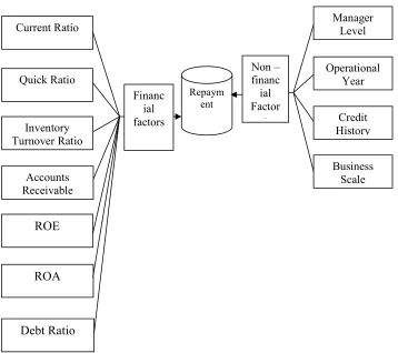
Figure 1. Model for the effect of independent variables affecting debt repayment capacity

Current Ratio

Quick Ratio

Inventory TurnoverRatio

Accounts Receivable

ROE

Operational Year

Credit History

Business Scale

ROA

Debt Ratio

Repaym ent

Financ ial factors

Non – financ

ial Factor

s

(5)

5

2.2.2. Select variables in the model

The topic uses set of data including of 240 observations sample. Using SPSS software to clean data and use Binary logistics regression model to find out the impact of each individual element of the customer affects their ability to pay debts.

Dependent variable

Y: Repayment

Y = 1: If the customer is able to repay Y = 0: If the customer is unable to repay

Independent variables

Table 2. Information of independent variables

Ordinal

Numbers Variables Scale Hypothesis Symbol

1 Current Ratio Current assets

Short − term liabilities + X1

2 Quick ratio Current assets − Inventory

Short − term liabilities + X2

3 Inventory Turnover Ratio

Cost of goods sold

Average of Inventory + X3

4 Accounts Receivable Turnover

Revenue

Average of Accounts Receivable + X4

5 Debt Ratio Total liability

Total Assets - X5

6 Bank loans tens of billion dong - X6

7 ROA Profit after taxes

Total Assets + X7

8 ROE Profit after taxes

Owners’ equity + X8

9 Manager Level 0: Under university - X9

1: After university +

10 Credit history 0: repayment in full and on time + X10

(6)

6

11 Operational Year 0: Under three year - X11

1: After three year +

12 Business scale

0: Small and medium

enterprises - _X₁₂

1: Big enterprises +

3. Result

3.1. Logistic model

Table 3. Variables in the Equation

B S.E Wald df Sig. Exp(B)

Current Ratio 4.293 1.613 7.084 1 .008 73.161

Quick ratio 3.139 1.489 4.441 1 .035 23.076

Inventory Turnover Ratio 2.370 1.051 5.090 1 .024 10.702

Accounts Receivable Turnover .930 .455 4.178 1 .041 2.534

Debt Ratio -2.349 1.134 4.292 1 .038 .095

Bank loans -.262 .125 4.427 1 .035 .769

ROE .115 .057 4.097 1 .043 1.122

ROA .340 .159 4.582 1 .032 1.405

Manager Level 3.342 1.441 5.378 1 .020 28.269

Operational Year 2.997 1.433 4.372 1 .037 20.032

Credit History -2.685 1.348 3.968 1 .046 .068

Business scale 2.365 1.183 4.001 1 .045 10.648

Constant -19.141 6.709 8.139 1 .004 .000

(7)

7

The general logistic regression equation has the form:

Ln(odds) = 𝐵 + 𝐵 𝑋 + 𝐵 𝑋 + 𝐵 𝑋 + 𝐵 𝑋 + 𝐵 𝑋 + 𝐵 𝑋 + 𝐵 𝑋 +

𝐵 𝑋 + 𝐵 𝑋 + 𝐵 𝑋 + 𝐵 𝑋 + 𝐵 𝑋

From the logistic regression analysis table, we can write the logistic equation in the economic direction as follows:

Ln(odds) = -19.141 + 4.293* X1 + 3.139* X2 + 2.370* X3 + 0.930* X4 - 2.349* X5 -

0.262* X6 + 0.115* X7 + 0.340* X8 + 3.342* X9+ 2.997* X10- 2.685* X11+ 2.365* X12

3.2. Determining influence level of independent variables on debt repayment (Dependent)

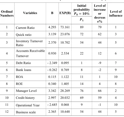
Table 4. The influence level of independent variables on debt repayment

Ordinal

Numbers Variables B EXP(B)

Initial probability

𝑷𝟎 = 𝟏𝟎%

Level of increase

or decreas

e%

Level of influence

𝑷𝟏

1 _{Current Ratio} 4.293 73.161 89 79 1

2 _{Quick ratio} 3.139 23.076 72 62 3

3 Inventory Turnover

Ratio 2.370 10.702 54 44 5

4 Accounts Receivable

Turnover 0.930 2.534 22 12 6

5 Debt Ratio - 2.349 0.095 1 -9 7

6 Bank loans - 0.262 0.769 8 -2 9

7 ROA 0.115 1.122 11 1 10

8 ROE 0.340 1.405 14 4 8

9 Manager Level 3.342 28.269 76 66 2

10 Credit history 2.997 20.032 69 59 4

11 _{Operational Year} - 2.685 0.068 9 -1 10

12 _{Business scale} 2.365 10.648 54 44 5

(8)

8

3.3. Inspection system of the model

3.3.1. Wald lnspection

Performing Binary Logistics regression analysis with SPSS (Sig <0.05), we get the following results:

Current Ratio 4.293 1.613 7.084 1 .008 73.161

Quick ratio 3.139 1.489 4.441 1 .035 23.076

Inventory Turnover Ratio 2.370 1.051 5.090 1 .024 10.702

Accounts Receivable Turnover .930 .455 4.178 1 .041 2.534

Debt Ratio -2.349 1.134 4.292 1 .038 .095

Bank loans -.262 .125 4.427 1 .035 .769

ROE .115 .057 4.097 1 .043 1.122

ROA .340 .159 4.582 1 .032 1.405

Manager Level 3.342 1.441 5.378 1 .020 28.269

Operational Year 2.997 1.433 4.372 1 .037 20.032

Credit History -2.685 1.348 3.968 1 .046 .068

Business scale 2.365 1.183 4.001 1 .045 10.648

Constant -19.141 6.709 8.139 1 .004 .000

Source: Data analysis results from SPSS

From the above Logistics regression analysis results, we find that the value of the sig significance level of the independent variables is all <0.05, so the independent variables in the Binary logistics regression model have a correlation with the dependent variable is Repay. The statistical significance level of the above regression coefficients has a reliability of over 95%, the sign of the regression coefficients is consistent with the initial hypothesis

(9)

9

Table 6. Omnibus Tests of Model Coefficients

Chi-square

df

Sig.

Step

158.912

12 .000

Block

158.912

12 .000

Model

158.912

12 .000

Based on the results of testing the suitability of the model, we have sig <0.05 so the general model shows the correlation between the dependent variable and the independent variables in the model are statistically significant with confidence intervals above 99%

3.3.3. Testing the explanation level of the model

Table 7. Model Summary

Step

-2 Log

likelihood

Cox & Snell R

Square

Nagelkerke R

Square

1

33.508

a

_.531

_.885

a. Estimation terminated at iteration number 10 because parameter estimates changed by less than .001.

Explanatory coefficient of model: R2 Nagelkerke = 0.885. This means that 88.5% of the variation of the dependent variable is explained by 12 independent variables in the model, the rest is due to other factors.

3.3.4. Testing the level of predicting the accuracy of the model

Table 8. Classification Tablea

Observed

Predicted

Repay

_Percentage

Correct

unable to pay

debts

able to pay debts

Repay

Unable to pay debts_{Able to pay debts}

31

5

86.1

3

171

98.3 Overall Percentage

96.2

(10)

10

- In 36 responses, individuals who are unable to pay debts, the forecasting model is exactly 31, so the correct rate is 86.1%.

- In 174, the individuals who can pay the debt, the forecasting model is exactly 171, so the correct rate is 98.3%.

The correct forecast rate of the entire model is 96.2%

4. Discussion

Current Ratio 4.293 1.613 7.084 1 .008 73.161

Quick ratio 3.139 1.489 4.441 1 .035 23.076

Inventory Turnover Ratio 2.370 1.051 5.090 1 .024 10.702 Accounts Receivable Turnover .930 .455 4.178 1 .041 2.534

Debt Ratio -2.349 1.134 4.292 1 .038 .095

Bank Loans -.262 .125 4.427 1 .035 .769

ROE .115 .057 4.097 1 .043 1.122

ROA .340 .159 4.582 1 .032 1.405

Manager Level 3.342 1.441 5.378 1 .020 28.269

Operational Year 2.997 1.433 4.372 1 .037 20.032 Credit History -2.685 1.348 3.968 1 .046 .068

Business scale 2.365 1.183 4.001 1 .045 10.648

Constant -19.141 6.709 8.139 1 .004 .000

Source: Data analysis results from SPSS 4.1.Current Ratio

B1= 4.293, P0 =10%, 𝑒 = 𝑒 . = 73.161

P1 = ×

( ) =

. × .

. ( . ) =

.

. = 0.89

If the probability of initially repayment is 10%, when other factors unchanged, if the short-term payment index of the enterprise increases by 1 unit, the probability of paying the debt of that enterprise is 89% (increase up to 79% from the initial probability of 10%)

4.2. Quick ratio

B2= 3.139, P0 =10%, 𝑒 = 𝑒 . = 23.076

P1 = ×

( ) =

. × .

. ( . ) =

.

(11)

11

If the initially probability of repayment is 10%, when other remain factors unchanged, if the quick ratio of the enterprise increases by 1 unit, the probability of repaying the enterprise's debt is 72% (up to 62 % of initial probability is 10%)

4.3. Inventory Turnover Ratio

B3= 2.370, P0 =10%, 𝑒 = 𝑒 . = 10.702

P1 = ×

( ) =

. × .

. ( . ) =

.

. = 0.54

If the initial probability of repayment is 10%, when other remain factors unchanged, if the Inventory Turnover Index increases by 1 unit, the probability of repayment debt is 54% (up to 44 % of initial probability is 10%)

4.4. Accounts Receivable Turnover

B4= 0.930, P0 =10%, 𝑒 = 𝑒 . = 2.534

P1 = ×

( ) =

. × .

. ( . ) =

.

. = 0.22

If the initial probability of repayment is 10%, when other remain factors unchanged, if the Receivable Turnover Index increases by 1, the probability of repayment debt is 22% (up 12% compared to the initial probability of 10%)

4.5. Debt Ratio

B5= -2.349, P0 =10%, 𝑒 = 𝑒 . = 0.095

P1 = ×

( ) =

. × .

. ( . ) =

.

. = 0.01

If the initial probability of debt repayment is 10%, when other remain factors unchanged, if the debt ratio of the enterprise increases by 1, the individual's probability of repayment debt is 1% (reduction 9% compared to the initial probability 10%)

4.6. Bank Loans

B6= -0.262, P0 =10%, 𝑒 = 𝑒 . = 0.769

P1 = ×

( ) =

. × .

. ( . ) =

.

. = 0.08

If the initial probability of repayment is 10%, when other remain factors unchanged, if the business borrows more than 10 billion VND, the probability of repayment debt is 8% (lower than 2% compared to the initial probability 10%).

4.7. ROE

B7= 0.115, P0 =10%, 𝑒 = 𝑒 . = 1.122

P1 = ×

( ) =

. × .

. ( . ) =

.

(12)

12

If the initial probability of repayment is 10%, when other remain factors unchanged, if the ROE of the business increases by 1, the probability of repayment debt of that business is 11% (up 1% compared to initial probability is 10%).

4.8. ROA

B8= 0.340, P0 =10%, 𝑒 = 𝑒 . = 1.405

P1 = ×

( ) =

. × .

. ( . ) =

.

. = 0.14

If the initial probability of repayment is 10%, when other remain factors unchanged, if the ROA of the business increases by 1, the probability of repayment debt of that business is 14% (up 4% compared with initial probability is 10%).

4.9. Manager Level

B9= 3.342, P0 =10%, 𝑒 = 𝑒 . = 28.269

P1 = ×

( ) =

. × .

. ( . ) =

.

. = 0.76

If the probability of repayment is initially 10%, when other remain factors unchanged, if the manager level of business increases by 1 level, the probability of repaying the debt of that enterprise is 76% (up 66% compared with initial probability is 10%)

4.10. Operational Year

B10= 2.997, P0 =10%, 𝑒 = 𝑒 . = 20.032

P1 = ₍× ₎ = _{. (}. × . _. ₎ = ._. = 0.69

If the initial probability of repayment is 10%, when other remain factors unchanged, if the number of founded years of enterprise increases by 1 year, the probability of repaying the debt of that enterprise is 69% (up 59% compared with initial probability is 10%)

4.11. Credit history

B11= -2.685, P0 =10%, 𝑒 = 𝑒 . = 0.068

P1 = ×

( ) =

. × .

. ( . ) =

.

. = 0.09

If the initial probability of repayment is 10%, when other remain factors unchanged, if the business has a bad credit history, the probability of repaying the debt of enterprise is 9% ( Reduction 1% compared with initial probability is 10%).

4.12. Business scale

B12= 2.365, P0 =10%, 𝑒 = 𝑒 . = 10.648

P1 = ×

( ) =

. × .

. ( . ) =

.

(13)

13

If the initial probability of repayment is 10%, when other remain factors unchanged, if the enterprise has a larger Scale, the probability of repayment of that debt is 54% (Increase 44% compared with initial probability is 10%).

5.Conclusions

Credit risks bring huge consequences for banks. However, facing it is inevitable for every bank, especially in the context of fierce competition nowadays.

Logistic model can support bank managers have an additional tool to analyze and identify businesses are in danger of losing their ability to repay, while the model indicates factors that strongly affect risk Credit for managers to have appropriate focus policies

However, the Logistic model is only effective when the analytical data is standard actual data.

REFERENCES

[1]. Hoang Trong, Chu Nguyen Mong Ngoc (2008), Analyze research data with SPSS, Hồng Ðức Publication.

[2]. Donald J. Bowersox, David J. Closs (2001), Logistical Management: The Integrated Supply Chain Process, Michigan State University, United States

[3]. J. Scott Long & Jeremy Freese (2001), Regression models for categorical dependent variables using Stata, A Stata Press Publication

[4]. Maddala, GS (1983), “Limited dependent and qualitative variables ineconometrics”, Cambridge University Press

[5]. Thomas Goldsby, Robert Martichenko, Robert O. Martichenko (2005), Lean Six SIGMA Logistics: Strategic Development to Operational Success, United States.