A Numerical Method -High Accuracy Solution to Singular Differential Equations

(1)

Double-Blind Peer Reviewed Refereed Open Access International e-Journal - Included in the International Serial Directories Aryabhatta Journal of Mathematics and Informatics

http://www.ijmr.net.in email id- irjmss@gmail.com Page 284

A Numerical Method -High Accuracy Solution to Singular Differential Equations

Y.Rajashekhar Reddy

Assistant Professor, Department of mathematics

JNTUniversity college of Engineering Jagitial, Nachupally (kondagattu) Karimnagar-505501,Telangana State, India

Abstract:Recursive form of B-spline based collocation method is developed and applied to the second order singular differential equation with Neumann’s boundary conditions. Quadratic B-spline collocation is used to find the numerical solution of second order singular differential equation and compared the solution with the analytic and cubic B-spline collocation solution. The improvement intheaccuracy of thesolutionis seen when cubic B-spline collocation is used. Quadratic and cubic B-spline collocation methods are tested for its efficiency and stability. Degree of the basis function is increased by onein the present method and applied to solve secondorder singular differential equations with Neumann’s boundary conditions. Results of considered Numerical examples show theimprovement inaccuracy of the approximate solution as increased the degree of the basis function.

Keywords

Collocation method, B-splines, Singular differential equations, Neumann’sboundary conditions

1. Introduction

In recent years, many numerical methods are developed to solve singular differential equations with Neumann- Dirchlet’s boundary conditions. The methods include like B-spline collocation method [13], finite difference method [4], kernel space [5, 6] sinccollocation method [7] and predictor and corrector method [8] and many more. The B-spline based collocation method is used to evaluate boundary value problems including singular boundary value problems [9].

Decreasing the mesh size and raising the degree of the basis functionsare able to improvethe accuracyof an approximation solution.

However, it is observed from the recent literature that B-spline basis functions are derived using fixed equidistant space for a particular degree only. If the recursive formulation given by Carl.De boor [12] is applied, the basis function evaluation can be generalized and without fixing the degree of the basis function can be used in collocation method for uniform or non uniform mesh sizes.

In this text, after defining the B-spline basis function recursively,the B-spline collocation method is described and formulated. The improvement in accuracy of the methodis demonstrated by usingthe third degree B- spline basis function instead of second degree B- spline basis function inthe B-spline based collocation methodto secondorder singular differential equations with Neumann’s boundary conditions.

Considering second order linear differential equations with variable coefficients

)

(

)

(

)

(

₂

1 2 2

x

R

U

x

Q

k

dx

dU

x

P

k

dx

U

d

_

_

, axb …… (1)

with Neumann’s boundary conditions

U

'

(

a

)



d

1 ,

U

(

b

)



d

2

where

2

1 ,

2 ,

1 ,

,

b

d

k

and

k

(2)

Let





 



1

2

,

(

)

(

n

i

p i i

h

_x

_C

_N

_x

U

……. (2) ,where

C

_i’s are constants to be determined and

N

i,p

(

x

)

are

B-spline basis functions, be the approximate global solution to the exact solution

U

(x

)

of the considered second order singular differential equation (1).

2.1B-splines

In this section, definition and properties of B-spline basis functions [1, 2] are given in detail. A zero degree and higher degree B-spline basis functions are defined at

x

_i

recursively over the knot vector space

X



{

x

₁

_,

x

₂

_,

x

₃

...

x

_n

_

₁

,

x

_n

}

as

0 )

if

p



i

1 )

(

,

x



N

_i _p

if

x



(

x

_i

,

x

_i__i

)

N

_i_,_p

(

x

)



0 if

x



(

x

_i

,

x

_i__i

)

1 )

if

p



ii

(

)

(

)

₁_, ₁

(

)

1 1

,

N

x

N

x

N

_i _p

i p i

p i p

i i p i

i p

i  

  

  











………. (3)

where p is the degree of the B-spline basis function and

x

is the parameter belongs to

X

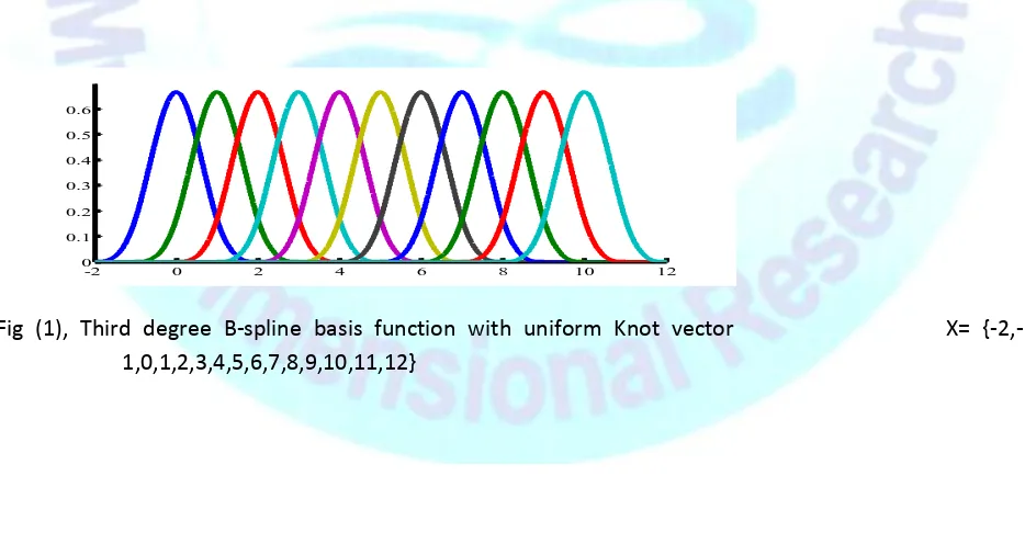
.When evaluating these functions, ratios of the form 0/0 are defined as zero

Fig (1), Third degree B-spline basis function with uniform Knot vector X= {-2,- 1,0,1,2,3,4,5,6,7,8,9,10,11,12}

-2 0 2 4 6 8 10 12

(3)

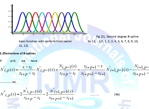
Fig (2), Second degree B-spline basis function with uniform Knot vector X= {-2, - 1,0, 1, 2, 3, 4, 5, 6, 7, 8, 9, 10, 11, 12}

2.2Derivatives of B-splines

If p=3, we have

1

1 )

(

1 ,

1 )

(

1 ,

1 '

1

1 )

(

1 ,

)

(

1 ,

'

)

(

,

'







































i

x

p

i

x

p

i

N

x

p

i

N

i

x

p

i

x

p

i

x

i

x

p

i

x

p

i

N

x

p

i

N

i

x

p

i

x

i

x

p

i

N

……… (4a)

1

1 )

(

1 ,

1 '

2 )

(

1 ,

'

2 )

(

,

''



















i

x

p

i

x

p

i

N

i

x

p

i

x

p

i

N

x

p

i

N

………… (4b)

In the above equations, the basis functions are defined as recursively in terms of previous degree basis function i.e. the pth degree basis function is the combination of ratios of knots and (p-1) degree basis function. Again (p-1)th degree basis function is defined as the combination ratios of knots and (p-2) degree basis function. In a similar way every B-spline basis function of degree up to (p-(p-2)) is expressed as the combination of the ratios of knots and its previous B-spline basis functions.

The B-spline basis functions are defined on knot vectors. Knots are real quantities. Knot vector is a non decreasing set of Real numbers. Knot vectors are classified as non-uniform knot vectors, uniform knot vector and open uniform knot vectors. Uniform knot vector in which difference of any two consecutive knots is constant is used for test problems in this paper. Two knots are required to define the zero degree basis function .In a similar way, a pth degree B-spline basis function at a knot have a domain of influence of (p+2) knots. B-spline basis functions of degree one and degree two over uniform knot vector are shown graphically below in figures (1) and (2).

-2 0 2 4 6 8 10 12

(4)

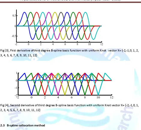
Fig (3), First derivative ofthird degree B-spline basis function with uniform Knot vector X= {-2,-1,0, 1, 2, 3, 4, 5, 6, 7, 8, 9, 10, 11, 12}

Fig (4), Second derivative of third degree B-spline basis function with uniform Knot vector X= {-2,-1,0, 1, 2, 3, 4, 5, 6, 7, 8, 9, 10, 11, 12}

2.3 B-spline collocation method

Collocation method is widely used in approximation theory particularly to solve differential equations .In collocation method, the assumed approximate solution is made it exact at some nodal points by equating residue zero at that particular node. B-spline basis functions are used as the basis in B-spline collocation method whereas the base functions which are used in normal collocation method are the polynomials vanishes at the boundary values. Residue which is obtained bysubstituting equation (2) in equation (1) is made equal to zero at nodes in the given domain to determine unknowns in (2).Let

[

a

,

b

]

be the domain

of the governing differential equation and is partitioned as

}

,

1 ...

2 ,

1 ,

0 {

a

x

_n

x

_n

b

X



_



with equal length

n

a

b

h





of

n

-sub domains.

The

x

_i

'

s

are known as nodes, the nodes are treated as knots in collocation spline method where B-spline basis functions are defined and these nodes are used to make the residue equal to zero to

-2 0 2 4 6 8 10 12

-0.5 0 0.5

-2 0 2 4 6 8 10 12

(5)

determine unknowns

C

_i

'

s

in (2), two extra knot vectors are taken into consideration beside the domain of problem both side when evaluating the second degree B-spline basis functions at the nodes.

Substuiting, the approximate solution (2) and its derivatives in (1).

)

(

)

(

)

(

₂ 1 2 2

x

R

U

x

Q

k

dx

dU

x

P

k

dx

U

d

h h h





i.e.

)

(

)

(

)

(

)

(

)

(

)

(

1 2 , 2 1 2 , ' 1 1 2 ,

''

_x

_k

_P

_x

_C

_N

_x

_k

_Q

_x

_C

_N

_x

_R

_x

N

C

n i p i i n i p i i n i p i

i













         …… (5)

Equation (5) which is evaluated at

x

_i

'

s

,i=0, 1, 2,....n-1 gives the system of (n-1) × (n+1) equations in which (n+1) arbitrary constants are involved. Two more equations are needed to have (n+1) × (n+1) square matrix which helps to determine the (n+ 1) arbitrary constants. The remaining two equations are obtained using

1 1

2

,

(

)



d



   n i p i i

N

a

C

, ……….… (6)

2 1

2

,

(

)



d



   n i p i i

N

b

C

, ….……… (7)

Now using all the above equations (5), (6), (7) i.e. (n+1) a square matrix is obtained which is diagonally dominated matrix because every second degree basis function has values other than zeros only in three intervals and zeros in the remaining intervals, it is a continuing process like when one function is ending its effect in its surrounding region than other function starts its effectiveness as parameter value changing. In other words, every parameter has at most under the three (p=2) basis functions. Thesystems of equations are easily solved for arbitrary constants Ci’s. Substuiting these constants in (2), the

approximation solution is obtained and used to estimate the values at domain points.Absolute Relative error is evaluated by using the following relationship in exact and approximate solutions

Absolute Relative Error =

t

xa

U

appro

U

t

xa

U

c

e

c

e



3. Numerical Experiments

The effectiveness of the present method is demonstrated by considering the various examples Example 1:Consider a singular boundary value problem given

5 .

5 )

1 (

,

0 )

0 (

,

1

0 ,

2 )

(

4

2 _'

_'

''

_

_U

_

_U

_x

_

_

_

_x

_

_U

_

_U

_

x

U

The exact solution is

2 sinh

)

2 sinh(

5

5 .

0 )

(

x

U





. The domain is divided into equal intervals and

(6)

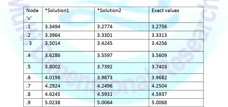
and third degree B-spline basis functionsin collocation method respectively and compared with the exact solution for mesh size h=0.100. It isobserved from the table1that the solution2 is veryclose to the exact solution as the solution1 can accomplish the same by taking very less mesh size. Increasing degree of basis function is easy then continuously attempting to increase interpolating points. Maximum absolute relative error for solution2 is 0.0017 for the 15 interpolating points whereas the same maximum absolute error for the solution1is achieved by taking the 201interpolating points.

Fig (5), Comparison of second and the third degree B-spline collation solutions with the exact solution for mesh size h=0.100 *solution1 is obtained by using the second degree B-spline basis function in collation method whereas *solution2 is the solution by using the third degree B-spline basis function in collation method.

Table 1Computed values and exact values at different nodes with mesh sizes ‘h=0.100’

Example 2: The exact solution of another singular boundary value problem considered below

0 0.2 0.4 0.6 0.8 1

3 3.5 4 4.5 5 5.5

*Solution1 Exact solution *Solution2

Node ‘x’

*Solution1 *Solution2 Exact values

.1 3.3494 3.2774 3.2756

.2 3.3964 3.3301 3.3313

. 3 3.5014 3.4245 3.4256

.4 3.6286 3.5597 3.5609

.5 3.8002 3.7392 3.7403

.6 4.0198 3.9673 3.9682

.7 4.2924 4.2496 4.2504

.8 4.6245 4.5931 4.5937

(7)

0 )

1 (

0 )

0 (

'

,

2 )

2

8 (

8 '

1 ''

_







U

an

d

U

x

U

x

U

is

)

2

8

7 log(

2 )

(

x

U





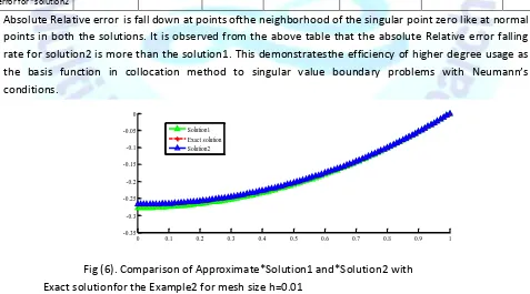
The following below figures 6, 7and 8 gives the comparison of solution1 and solution2 with the exact solution for example.2 for different mesh sizes ‘h’.Decreasing mesh size improves the approximation solutions as well as consistently moving to converge with exact values very well. The convergence rate is high for solution2 when compare with soltion1.This shows the consistency of the method as the higher degree is used as basis function in evaluating second order singular differential equations with Neumann’s boundary conditions.

Table2 gives the relativeerror of the nodes which are in the neighborhood of the singularpoint zero for both the solutions

Nodes close to singular point x=0

.0100 .0050 .0025 .001 .0007 .0005 .0003

Absolute Relative error for *solution1

.001001 0.000479 0.000234 .000092 .000061 .000045 .000022

Absolute Relative error for *solution2

.00000405 .00000101 .0000002 .000000040 .000000018 .0000000101 .0000000043

Absolute Relative error is fall down at points ofthe neighborhood of the singular point zero like at normal points in both the solutions. It is observed from the above table that the absolute Relative error falling rate for solution2 is more than the solution1. This demonstratesthe efficiency of higher degree usage as the basis function in collocation method to singular value boundary problems with Neumann’s conditions.

Fig (6). Comparison of Approximate*Solution1 and*Solution2 with Exact solutionfor the Example2 for mesh size h=0.01

0 0.1 0.2 0.3 0.4 0.5 0.6 0.7 0.8 0.9 1

-0.35 -0.3 -0.25 -0.2 -0.15 -0.1 -0.05 0

(8)

Conclusions

The effectiveness of the proposed method is illustrated by considering two numerical examples. Thehigh degree B-spline basis function is usedin collocation method and comparedwith lessdegree B-spline basis function. The high accuracy is achieved by raising the degree of the basis function very wellwith less interpolating points and performance of the method with high degree basis function at nearby singular points is as ordinary points. Theconvergence rate is high when used low degree B-spline basis function in collocation methodand time is savedbecause more interpolating points are required to get the same level of accuracywhen used lowdegree B-spline basis function in collocation method..This method may be applied to different types of some more singular boundary value problems for its efficiency

References

*1+Hughes, T.J.R., Cottrell, J.A. and Bazilevs, Y. ‘‘Isgeometric analysis: CAD, finite elements, NURBS, exact geometry and mesh refinement’’,Comput.Methods Appl. Mech. Engg., 194(39–41), pp. 4135– 4195 (2005).

*2+ David F.Rogers and J.Alan Adams, “Mathematical Elements for Computer Graphics”, 2nd ed., Tata McGraw-Hill Edition, New Delh.

[3] C. de Boor and K. H¨ollig.B-splines from parallelepipeds. J. Analyse Math., 42:99– 15, 1982

[4] R.K. Pandey and Arvind K. Singh, On the convergence of a finite difference method for a class of singular boundary value problems arising in physiology, J. Comput. Appl. Math 166

(2004) 553-564.

[5] Geng, F.Z. and Cui, M.G. (2007) Solving Singular Nonlinear Second-Order Periodic Boundary Value Problems in theReproducing Kernel Space. Applied Mathematics and Computation, 192, 389-398.

[6] Li, Z.Y., Wang, Y.L., Tan, F.G., Wan, X.H. and Nie, T.F. (2012) The Solution of a Class ofSingularly PerturbedTwo-Point Boundary Value Problems by the Iterative Reproducing Kernel Method.

Abstract and Applied Analysis, 1-7

[7] Mohsen, A. and El-Gamel, M. (2008) On the Galerkin and Collocation Methods for Two Point Boundary Value ProblemsUsing Sinc Bases. Computers and Mathematics with Allications, 56, 930-941.

[8] AbdalkalegHamad, M. Tadi, MilojeRadenkovic (2014) A Numerical Method for Singular Boundary-Value Problems.Journal of Applied Mathematics and Physics, 2, 882-887.

[9] Joan Goh_, Ahmad Abd. Majid, Ahmad Izani Md. Ismail (2011) Extended cubic uniform B-spline for a class of singularboundary value problems.Science Asia 37 (2011): 79–82

[10] I. J. SCHOENBERG Contributions to the problem of approximation of equidistant data by analytic functions, Quart. Appl. Math. 4 (1946), 45-99; 112-141.

[11] H. B. CURRYA ND I. J. SCHOENBERG On Polya frequency functions IV: The fundamentalspline functions and their limits, J. Anal. Math. 17 (1966), 71-107.

(9)

[13]HikmetCaglar, NazanCaglar, Khaled Elfaituri(2006). B-spline interpolation compared with finite difference, finite element andfinite volume methods which applied totwo-point boundary value problems.Applied Mathematics and Computation 175 (2006) 72–79